STATISTICAL ANALYSIS OF DEMOGRAPHIC AND EDUCATION DATA FOR PROJECTING SCHOOL ENROLMENT IN INDIA
Item
- Title
-
STATISTICAL ANALYSIS OF DEMOGRAPHIC
AND EDUCATION DATA FOR PROJECTING
SCHOOL ENROLMENT IN INDIA
- extracted text
-
V
■
SEM/INDIA/1
Paris, September 1978
Original : English
UNITED NATIONS EDUCATIONAL
SCIENTIFIC AND CULTURAL ORGANIZATION
STATISTICAL ANALYSIS OF DEMOGRAPHIC
AND EDUCATION DATA FOR PROJECTING
SCHOOL ENROLMENT IN INDIA
Document prepared for the national training seminar on
methods for projecting school enrolment in India
New Delhi ,
20 November - 1 December 1978
i
i
Education Projections Unit
Division of Statistics on Education
Office of Statistics
PREFACE
*
Projection of the future number of pupils enrolled constitute the starting
point of quantitative educational planning, as they provide the basis for estimat
ing the future needs of teachers, classrooms and other facilities. While in develop
ing countries the need for such projections is well recognised, the national ser
vices responsible for their preparation do often not have sufficient personnel qua
lified in the statistical methods required. This is particularly true for- methods
which take adequately into account population variables and which are adapted to the
education and population data available in these countries.
The Unesco Office of Statistics, Paris, has since 1972 been engaged in prepar
ing education projections with special reference to developing countries. In the
course of this work, the need for specialized training in simple statistical methods
for quantitative analysis of the relationship between population growth and educa
tion requirements became evident. To meet this need the Office has, with the .finan
cial support of the UNFPA (United Nations Fund for Population Activities) undertaken
to arrange national training seminars on methods for projecting school enrolment, in
developing countries. The project includes four seminars per year during the three
year period 1977-1979. Its main objective is to develop a greater awareness in de
veloping countries of the need to take adequately into account population variables
when preparing educational plans.. This will be achieved by promoting the use of
statistical methods adapted to the education/population problems encountered and the
statistical data available in the countries participating in the project. Each semi
nar will last for about- 10 working days and is designed for around 30 participants,
• drawn to the extent possible from services responsible for educational statistics
and educational planning at. the regional and province level.
India is one of the four countries participating in the second year of this
project. The seminar in India will be held in New Delhi in the period 20 November - •
1 December, 1978. The purpose of the present document is to serve as a support for
the teaching at this seminar. Although self-contained, this document should be read
with this in mind since several topics which have only been touched upon here will
be dealt with in further detail during the sessions.
9
The seminar has been arranged jointly by the Unesco Office of Statistics and
the National Staff College for Educational Planners and Administrators New Delhi, in
co-operation with the Union Ministry of Education and Social Welfare, Government of
India. We should like to express our deep gratitude to the national authorities for
their help in supplying the statistical information required for preparing this
document.
Paris, September 1978
UNESCO OFFICE OF STATISTICS
(i)
TABLE OF CONTENTS
Page
1
...c
INTRODUCTION
2
.
PART I : POPULATION AND-1 EDUCAT ION IN -INDIA . .'. . . . . .
-------- ;—
,--- :—: : : r
.r
SECTION 1 • • POPULATION: • BASIC CONCEPTS OF DEMOGRAPHY
2
The sub j ec t-mattexJof •„ dsmgraphy .
The size of the population . . .... ... . .
The ratelofjpppulatipM1 'growth. in...India-.
Births
. 1.1.5 Deaths - . < .... . .
L.J.6 ;Lifectables--..
1.1.7 Migration
I. 1 .8 Population ’-ptctxx
x
1.1.1
1.1.2
1.1.3
1.1.4
c •:
2
2
5
6
8
11
12
13
1
'J? I
SECTION 2.:.DEMOGRAPHY AND EDUCATIONAL PLANNINGe -
C~t
3 •*.
r/
1 j.?/ .Cu
’
x- -■
-
. / .:i
Intreduction
—v. •.
Quality -of idem©graphic. ;data .. .I".. - ..... .
--- --1.2.3 The.geographical distribution^of . the population
1.2.4 The distribution of’ the. population by sex and age ...
1.2.5 Population of school:^age . ,
...... .i.
..
1.2.6 The burden imposed by the school population
1.2.7 Distribution of the labour; force by .economic '-sector .
1.2.8 Stock of education in the population
1.2^9- - Concluding; remarks on' Part' I . . 7.
.I..2?l
15
15
16
21
24
24
26
28
29
PART II : SCHOOL AGE POPULATION AND SCHOOL ENROLMENT RATTOS IN INDIA
SECTION !
ENROLMENT RATIOS' J 6.‘ ~
II.1.1 Introduction ..
II. 1.2 Def inition.. of enrolment ratios .
30
31
SECTION 2 :...THE EDUCATIONAL FLOW MODEL AND ITS USE IN PROJECTING
1
.RUTHRE ENROLMENT ' IN 'PRIMARY EDUCATION
II.2.1 Introduction...,.,.*
............
II. 2.2 Characteristics.' of~ educational ,flow models
11.2.3 Distinction between enrolment projections, forecasts and
targets'
A ...... ..........
11.2.4 The advantages of' mathematical models ....
11.2.5 The flow of students through an education cycle
11.2.6 Reconstruction of'the school history of a given cohort ...
11.2.7 Efficiency in education
.............
11.2.8 The role of education projections in educational
planning . .
-. ..................
11.2.9 Factors influencing the student-flow
; p- (ii)
36
37
37
38
39
45
48
50
50
II.2.10 Preparing an enrolment projection...
II.2.11 Projection of the age-group of admission age
II.2.12 Methods of projecting new entrants ...
II.2.13 Projection of transition rates
.....
II.2.14 Projection of enrolment in elementary education
II.2.15 . Tile Rstention Model or Grade Ratio Model ......
11.2.16 Sensitivity analysis
"
11.2.17 Concluding remarks on Part II . ............
51
52
52
60
..
...
..
..
..’bl
. . . 61
... 64
. 65
PART III ; THE CALCUBATION OF TEACHER REQUIREMENTS
•
..........
•• ■
- .
......
- •
> J *. 17.1
‘.'r
. SECTION J : CHARACTERISTICS OF THE TEACHING'STOCK
III.1.1
Introduction ....
Size and distribution of the teaching stock:in -India ...
66
66
SECTION 2, : PROJECTION OF TEACHER REQUIREMENTS
III.2.1
III.2.2
Introduction ,.
.V>. .J.... i;.\ ......... w;
Method based on the number of pupils and the pupil
. teacher ratio .......... ... * J......,
. .111.2,3. Method based on the number of pupils per class and hours
■ taught - by teachers
....,.
III.2.4p Projecting the: demand for new teachers
. .111,2.-5 Concluding remarks on Part III :..
• ••••••••• .4 £■•••••»••••••••.
PART TV
72
72
73
74
75
EXPENDITURE, ON EDUCATION- IN INDIA-
SECTION .1 . : THE ASSESSMENT OF NATIONAL EDUCATIONAL EXPENDITURE
IV. 1 JJ
IV.1.2
IV.1.3
IV.1.4
IV.1.5
Introduction;
.j.#.
Definitional problems ........................... e
Sources of educational finance
.
Educational expenditure in relation to economic
aggregates
J...9 o , a
Recent trends in expenditures by type .of education
77
77
78
79
80
SECTION 2 : COMPOSITION AND. DISTRIBUTION OF-EDUCATIONAL
EXPENDITURE .. .
.7
. ■ . ..----IV.2.1
IV.2.2
ANNEX
ANNEX
Alternative ways of disaggregating expenditure .....
Analysis by spending agency and administrative '
programme .... .7
...... .. .; .........
IV.2.3
Analysis by type of expenditure . ’
.......
IV.2.4
Analysis by level and specialisation
.... ’
IV.2.5
Analysis by geographical area
SECTION 3 : THE ANALYSIS OF EDUCATION COSTS
83
83
84
86
IV.3.1
IV.3.2
IV.3.3
IV.3.4
Introduction
..........
Opportunity cost
....
^Costing educational plans ...
Concluding remarks on Part IV
88
88
89
90
1 •* Curve fitting and the method of least squares
2 : Flow diagrams .............. , .
91
(iii)
83
97
POPULATION AND EDUCATION IN INDIA
PART I :
SECTION 1
POPULATION: BASIC CONCEPTS OF DEMOGRAPHY
«
1.1.1
The subject-matter of demography
Demography is the scientific study of certain characteristics of human popu
lations, particularly with respect to their magnitude, their change over time, and
their structures according to sex, age, occupation, geographical location and other
characteristics. Virtually all quan&itative analyses in educational planning depend
upon population information in one form or another. For this reason all educational
planners need an understanding of the basic concepts of demography - including an
appreciation of their limitations... We shall therefore review some of these concepts
in this section. However, as the main -objective of this seminar is to provide train
'■ • ing in education projection methods, this review will be partial and the readers are
referred to specialized literature on demography-, for further study of this topic.
Human populations undergo continuous change. The changes,, in the set of indivi
duals which make up the population may be divided into three, usually termed*By'"de
mographers the "vitaln” processes :
i
a)
b)
c)
births.
deaths
migration.
A
J
Before we examine how these vital processes may be measured
mental statistic:- the- si-z-e-of the population." '
I. 1.2
let us look at a funda
The size of the_ population
The main sources of information on population size - that is the state of a
population at a given time - are from censuses and registration systems. Censuses
involve the complete enumeration of all the inhabitants of a defined geographical
area. In.developed countries these have had a long and valuable history. In the
Uni_ed.Kingdom, for example, censuses of the population have been taken every tenth
year since 1801. They are, however, expensive to carry out and demand large numbers
of trained personnel for their satisfactory completion. Consequently, a number of
developing countries have yet to implement scientific population censuses. This is
not the case in
-- India
----- where
---- » a number of population censuses have been carried out.
w?16 1 sbows the absolute size of the Indian population in decennial Censuses
19 J I 19/1, and the average annual rates of population growth between the Censuses
(1). The table shows that over the seventy years 1901-1971 the population grew by
309.8 million. This represents a total percentage growth of 129.9^, at an average
annual rate of 1.2%.
(1)
The concept of the average annual growth rate is defined in 1.1.3 below.
2
MIUUO*J
Figure 1.
X’oo
Growth of Population in India 1901-1971 (millions)
9
3^0
-3oo
Zoo
0
r
V)
e“
Table 1.
6*
Population Size and Average Annual Rate of Growth in India, Decennial
Censuses 1901-1971.
Census date
Population
(millions)
1901
1911
1921
1931
1941
1951
1961
1971
238.4
252.1
251.3
279.0
Source :
Average Annual Rate of Growth
Between Censuses (%)
-0^-6.-0.-03 —
—1.05 —'
1.34
1.26
1.98
2.24
318.7
361.1
439.2
548.2 .
Statistical Abstract, India 1975, Central Statistical Organization,
Ministry of Planning, Table 5.
It may be noted that the highest inter-censal average annual growth rate of
2.24% occured during the most recent inter-censal period, 1961-1971. This high rate
however declined over the period 1971-1976. The Expert Committee on population pro
jections estimated that the 1976 population totalled 610.1 million (1)-. Over the 5
(1)
Statistical Pocket Book, India, 1977, Central Statistical Organization, Ministry
of Planning, p. 6; and Demographic Yearbook, 1976. United Nations, New York,
1977; Table 3.
- 3
year period 1971-1976 this represented an average annual growth rate of 2.16%. A
further projection for 1981 (1) has suggested that total population will be 672
million. This would represent a slight decline in the average annual growth rate to
2.1% over the total ten year period 1971-1981.
Projections of the Indian population were assessed by the United Nations in
1973 and are presented in Table 2. Three alternative sets of assumptions regarding
trends in the vital processes are made (See Section 1.1.8 of this paper). It should
be noted that even the low variant of the United Nations projections gives figures
higher than the recent estimates and projections made by the Indian national authori
ties and cited above.
Table 2.
United Nations Population Projections for India, 1970-1985 (millions)
Year
Low variant
(a)
Medium variant
(b)
High variant
(c)
1970
1975
1980
1985
543.1
610.4
683.6
757.4
543.1
613.2
694.3
782.9
543.1
613.9
697.6
795.3
2.24
2.47
2.54
Annual
average
growth
rate
19701985 (%)
Source:
World Population Projects as Assessed in 1973, Population Studies
No. 60, United Nations, New York, 1977, Tables 28, 30 and 31.
The average annual growth rate over the period 1970-1985 implied by the low
variant population projections is 2.24%, exactly the inter-censal rate actually
recorded between 1961 and 1971. However, taking 5—year periods separately, the
United Nations low variant implies a decline in the growth rate from 2.34% (1970-75)
to 2.05% (1980-85). The reader should note that these projections were prepared in
1973 and that they are currently being revised by the United Nations.
Although the size of the population indicates to the educational planner gene
ral orders of magnitude, by itself it represents information of only limited value.
This is because populations of similar size may differ greatly as to their past and
future dynamic behaviour (change over time) and in their structure (distribution by
age, sex or other characteristics). In the remainder of Section 1 we shall be mainly
concerned with the dynamic behaviour of population. In Section 2 we consider some of
the structural implications.
(1)
Country Report, India, Fourth Regional Conference of Ministers of Education
and those Responsible for Economic Planning in Asia and Oceania, Colombo 1978,
Chapter 1. Report prepared by the Ministry of Education and Social Welfare.
- 4
The rate of population growth in India
I. 1 .3
As has already been implied in the above discussion, the average annual rate
of growth is an important basic tool in demography. It should not be confused with
the total percentage growth of population over a period of time. To clarify the
distinction between these two concepts, let us consider the official projection of
total population from 548.2 million in 197! to. 672 million in 1981. This represents
a projected increase of 22.6% over the 10 year period. It is not an average annual
rate of growth. In fact, the average annual rate of growth which corresponds to a
total percentage growth of 22.6% over a 10 year period is 2.1%. Let us now see how
each of these figures has been calculated.
The total percentage growth of 22.6% over the period 1971-1981 has been calcu
lated by the following formula :
(1) percentage growth over the period = 100 —-
L°
where P
P
o
n
=
Population in the initial year "o”
=
Population in the final year ” n".
1
J
Hence, % growth over the period 1971-1981 -
100
672
548.2
L 518-2 J
%
22.6%.
The average annual rate of growth is calculated by formula 2 shown below. This
is in fact the standard formula for reckoning compound growth, where annual percen
tage increases are reckoned on the base not only on the original figure in Year 1
but also on compounded successive annual increments. It contrasts with the simple
rate of growth formula which adds a constant amount each year to the original. The
difference between a compound rate of growth and a simple rate of growth can readily
be illustrated by considering how a sum of 1000 rupees would grow in the face of 10%
rates of interest.
COMPOUND INTEREST
SIMPLE INTEREST
Accrued Capital
Sum
Annual Interest
(10% of original
capital)
1000
1 100
1200
1300
1400
100
100
100
100
100
1000
1100
1210
1331
1464.1
Accrued Capital
Year
Year 1
Year 2
Year 3Year 4
Year 5
Sum
Annual Interest
(10% of accrued
capital)
100
110
121
133.1
146.41
Population growth is of the compound variety and it is quite easy to see there
fore that one cannot simply divide the total percentage increase above (22.6%) by
the number of years (10) to arrive at the average annual rate of increase. Instead
the formula one uses to arrive at average annual rate of incr-ease is :
(2)
P
n
= P
■ (1
+ r)n
o
being the rate we want to calculate.
- 5 -
To calculate r from this formula we have to take logarithms and re-express the
formula as :
n
log P o
Pn
Q°g
<1 .
This can in turn be rearranged as
log Pn
-
Po
n
Qog (1 + rf| , or log
(1 + r)
log pn - log Pq
n
In the example under discussion,
p
P
672
n
548.2
o
10.
n
Thus :
log (1
r)
8.8274 - 8.7389
10
(1 + r)
1 .021
n
0.021
2.1%
EXERCISE I
Columns (a)> Cb) and (o) of Table 2 give the United Rations low3
medium and high variant projections respectively of the population
of India from 1970-1985. Using these figurescalculate for each
variant :
i) the total percentage growth over the period 1970-1980.
ii) the average annual rate of growth from 1970-1980.
Formula (1) and (2) should be used for calculations.
The rate of growth of the total population describes population change, but
does not explain it. For an understanding of the underlying factors giving rise to
this change, the vital processes must be analysed: births, deaths and migration.
1.1.4
Births
Crude birth rate
The crude birth rate of'’an area is defined as the number of live briths occuring in that area in a given time period, usually a year, divided by the population
of the area as estimated at the middle of the particular time period. The rate is
most often expressed in terms of "per 1000 of population".
(3)
Crude birth rate =
Number of live births in a year
Mid-year total population
- 6
x 1000
The crude birth rate in India in 1975 was 35.2 per thousand (1).
The crude birth rate is an elementary statistic which requires only global in
formation for its calculation. It is not calculated with any reference to the struc
ture of the population according to age or sex, even though it is the proportion of
women of child-bearing age in the population that largely determines present and
future population changes. Therefore a more refined measure of "fertility" is de
sirable.
Fertility rates
Fertility measures the rate at which a population augments itself by births
relating births to the number of females "at risk", that is, of child-bearing age.
Two fertility rates may be distinguished here, the general fertility rate and the
age-sepcific fertility rate.
(4)
the general fertility rate =
Number of live births in a year_______
Mid-year population of women of child-bearing age x 1000
The general fertility rate in India over the period ’ 1961-1971 was 193 (2). Often
"child-bearing age" is taken to be 15-49 years. It is called a "general" rate be
cause it attributes all births to all women within these age-limits. Clearly however
fertility is not constant over all years of child-bearing potential. A more disaggre
gated measure of fertility is the age-specific fertility rate.*
(5)
the age-specific fertility rate =
Number of live births born to women in a specified age-group in a year^jqqq
Mid-year population of women in the specified age-group
In calculating the age-specific fertility rate, potential mothers may be grouped by
single year of age or by age-groups of, e.g., 5 years. It need hardly be added that
the age of women is not the only factor affecting fertility. Fertility depends on
numerous other influences - social and cultural as well as physical - including
the availability and use of techniques of birth control, age at marriage, duration
of marriage, average time between births, and so on. It is important to note that
fertility rate calculations are based on the number of births occuring in a single
year. Obviously these rates may change quite considerably over time. A dynamic ana
lysis of population change must take account of both these changes and the second
vital process we have specified: deaths.
(1)
Dates supplied by national authorities from Sample Registration Scheme, Regis
trar General.
(2)
Ibid..
7
I. 1 .5
Deaths
The crude death rate of an area is defined analogously to the crude birth rate.
It is the number of deaths occurring in that area in a given time period, usually a
year, divided by the population of the area as estimated at the middle of the time
period :
(6)
crude death rate
Number of deaths in a year
Mid-year total population
x
1000
The crude annual death rate in India in 1975 was 15.9 per thousand (1). Over the
period 1961-1971 the rate was estimated to be 18.9 per thousand.
Deaths result, of course from a multitude of causes (some of which can, and some of
which cannot, in principle be influenced by public policies). The different agegroups in the population experience different rates of mortality from specified
causes. For this reason, the crude death rate is only a relatively clumsy tool for
the social planner. To further investigate the mortality experienced by a population,
deaths rates according to age may (data permitting) be usefully calculated.’
The age-specific death rate is defined as follows :
(7) age specific death rate
Number of deaths in a year in a specified age-group
Mid-year population in the specified age-group -x 1000
One commonly calculated age-specific death rate is the infant mortality rate
(8)
Infant mortality rate
Number of deaths below age 1 in a year
x 1000
Number of live births in the year
Because of the susceptibility of small babies to infection and their vulnerability'
vulnerability
to accidents this rate is generally much higher than other age-specific death rates
(until a great age is reached). It and the other age-specific rates up to the year
of entry into the school system, are of obvious importance to the educational plan
ner in projecting future school intake. According to national estimates the infant
mortality rate in India was 122 per thousand live births in 1971 (2).
Another basic demographic relation which may now be introduced is the crude
rate of natural increase. This measures the change in population size, due to births
and deaths, as a percentage of total population. (Note that it takes no account of
net migration: the difference between emigration and immigration). It is defined
as follows :
Number of births in a year minus
(9) Crude rate of natural increase = number of deaths in a year____
x 1000
Mid-year population in the year
(1)
Data supplied by national authorities from Sample Registration Scheme, Registrar
General. For 1971 the rate was estimated to be 14.9 per thousand.
(2)
Data supplied by national authorities. This figure for 1971 is also given in the
Demographic Yearbook 1976, (op. cit.), Table 4, though a few states were not
included.
- 8
w
Table 3 presents data for India (1961-1971) and selected world regions
(1965-1976). It can be seen that the crude birth and death rates in India were signi
ficantly higher than the world averages for the period 1965-1976. India’s rate of
natural increase at 23 per 1000 population was somewhat above the world figure of
19 per thousand, and very close to that of Asia as a whole (in which India is inclu
ded). It should be noted that the rates of natural increase (i.e., the differences
between crude birth and death rates) do not always exactly correspond to the figures
for the annual rate of population growth in the first column of the table. Discre
pancies may of course be due to error and differing methods of estimation, but the
third vital process, migration, if significant will cause a divergence between the
two rates.
Table 3.
Annual growth of population, crude birth and death rates and rate of
natural increase - India and selected regions, 1965-1976
Annual rate
of population
growth 7O
1965 - 1976
India (1)
Africa
Asia (2)
Europe
Latin America
North America
U.S.S.R.
World
Crude
birth rate
(per 1000)
1965-1976
Crude
death rate
(per 1000)
1965-1976
Rate of
natural
increase
(per 1000)
1965 - 1976
2.2
2.7
2.2
0.6
. 2.7
1 .0
1.0
41.9
46
36
16
38
17
18
18.9
20
14
10
10.
9
8
23
26
22
6
28
8
10
1.9
32
13
19
Source :
Data for regions derived from Demographic Yearbook, 1976, op. cit.. Table
1.
Notes
(1)
(2)
Data for India supplied by national authorities and refer to the
period 1961-1971.
Including India.
A feature of Table 3 in general is the marked difference between the crude rates
of natural increase experienced in the industrialized regions of Europe, North
America and the USSR and those ruling in the less developed regions of Africa, Latin
America and Asia (including India). The most recent estimate of the crude birth rate
supplied by Indian national authorities indicates a figure of 35.2 live births per
thousand population in 1975. This is well over twice the rate of 14.7 (1) experienced
in the United States in 1976, for example, though well below the rate of 49.5 (1)
estimated in Bangladesh over the period 1970-75.
(1)
Source : Demographic Yearbook 1976, op. cit., Table 4.
9
India’s crude death rate is high by world standards arid significantly higher
than that for Asia as a whole. The annual rate of population growth, at 2,2% was 0.3
percentage points above the world average, and very considerably above the European
rate of 0.6%. If the rate of 2.2% experienced over the decade 1961-1971 (1) were to
continue, one can calculate (using formula (2) above) that the Indian population
would double in 31.9 years. By way of contrast, Europe’s population would take 115.9
years to double.
EXERCISE II
On the basis of the data given In the first column of Table
use
formula (2) to calculate the number of years It will take for the
populations of the countries and regions listed In this table to double.
Table 4 presents data illustrating the wide variance between countries in in
fant mortality and fertility rates and life expectancy at birth (a concept explained
in 1.1.6. below). It can be seen that infant mortality and fertility rates show a
strong positive association (i.e. the higher the infant mortality, the higher the
fertility rate tends to be). Life expenctancy at birth tends to be relatively high
in countries in which infant mortality rates are low. The table reveals the relative
ly low expectancy of life at birth for both sexes in India. For example, at birth an
Indian female can expect over 30 years less life than her counterpart born in the
United States.
(1)
According to data published in Statistical Pocket Book, 7India 1977, the rate over
the later period 1966-1976 was 2.15%, i.e. marginally lower.
10
Table 4.
Fertility rates, infant mortality rates, and life expectancy at birth ;
India and selected countries, 1970 - 1975
Fertility
rate
(per 1000) (1)
____ (a)
India
Argentina
Congo
Finland
Indonesia
U.S.A.
U.S.S.R.
136.7
94.2
178.5
47.6
175.7
60.4
55.5
(2)
(5)
(7)
(8)
(9)
(8)
Infant
mortality
rate
(per 1000)
(b)
122
59.0
180.0
10.2
125.0
16.7
27.7
(3)
(6)
(7)
(9)
(10)
(9)
(9)
Life expectancy
at birth
Male■
r- Female
(years)
(c)
(d)
47.1
(4)
65.2
41.9
66.6 (5)
47.5 (H)
68.2 (9)
64.0 (12)
45.6 (4)
71.4
45.1
74.9 (5)
47.5 (11)
75.9 (9)
74.0 (12)
Source :
India, column (a) Demographic Yearbook, 11976,r Table 4; column (b) Sample
Registration Scheme, Registrar General; columns (c) and (d) Statistical
Abstract 1975, Table 9.
All other countries, Demographic Yearbook, 1976, op. ,cit., Table 4.
Notes
(1) For India and USSR, per 1000 females aged 10—49 at year mid-point, For
all other countries, per 1000 females aged 15-49 at year mid-point.
(2) 1958-59. Estimate for rural India, based on results of National
Sample Survey
(3) 1971
(4) Based on 1% sample, 1971
(5) 1972; (6) 1970; (7) 1960-61; (8) 1973; (9) 1974;
(10) 1962; (11) 1960; (12) 1971-72.
1.1 .6
Life tables
The life table is ian analytical tool of great importance in demographic analy
sis . It presents the life-history of a hypothetical cohort of individuals"from birth
(though it could commence at any age) to their eventual death.
cohort is a set of individuals possessing some common characteristic. In this
case, the characteristic is a common year of birth. In later sections of this paper,
we shall consider cohorts of individuals flowing through the educational system;
and in that analysis, cohorts may be distinguished by their age or by their common
school grade in the initial year of the flow analysis.
A cohort of individuals bom in a particular year is gradually diminished, year
by year, by death, until all members have died. A life table may be a historical life
table, based on the observation through time of the mortality experienced by a real
cohort of individuals. Such tables are however of relatively little value compared
with life tables constructed by applying current mortality rates by age to a theoretical cohort of, say, 1000 persons. The construction of such tables requires a consi
derable amount of information, and they are not available for all countries. However,
if such tables can be drawn up, valuable indices may be estimated from them. These
include :
a) probabilities of death and survival for individuals at particular ages or periods.
11
b) life expectancies at particular ages: the average number of years that persons
at particular ages can be expected to live, i.e. will live on average if current
mortality rates continue into the future.
Life expectancy at birth is a widely-used indicator in comparative studies.
Low life expectancy at birth is usually associated with high infant and childhood
mortality rates. Even where a country’s life expectancy at birth is low by internataional standards, it is often the case that life expectancy at age 10 is signifi
cantly higher and indeed comparable with countries at relatively advanced levels of
socio-economic development. This is because of the very high rates of infant and early
childhood mortality. Once an individual has survived this particularly risky period
of his life, he may expect to survive for a number of years comparable with his surviving contemporaries in other countries having much lower rates of childhood morta
lity.
1.1.7
Migration
The third major component explaining population change together with births and
deaths is, of course, migration. Clearly in analysing past population change, and
in projecting future change, rates of emigration and immigration may play an important
role. For detailed manpower and educational planning, age-specific rates of migration
would obviously be desirable and it would also be useful to know the education level
of both immigrants and emigrants. Statistical information on the number, age and
educational level of both immigrants and emigrants can rarely be obtained even in
highly developed industrial countries having relatively comprehensive systems of data
collection. Such details were unfortunately not available in the preparation of this
study.
However, population migration within a country (’’internal migration”) may be of
considerable importance for economic and social planning.- In particular the phenomenon
of population movement from rural to urban areas has, historically, been invariably
associated with economic development. The process is currently being observed in India
and may be expected to continue in the long term. The development will have potential
ly important consequences for educational planning, particularly through its effects
on enrolment rates and other rates such as those of intake and drop out, to be dis
cussed later in this paper. A research study (1) in investigating rural-urban migra
tion in Greater Bombay and its implications for educational planning found that the
more educated and the more skilled in rural areas tended to migrate to urban areas.
This inevitably tends to depress rural areas and creates a problem similar to that
of the brain drain . The study also found that rural migrants endeavoured to improve
their educational qualifications after migrating to urban areas. A further finding
with important implications for population growth and educational planning was that
rural migrants had a lower fertility than non—migrants, but a higher fertility than
urban non—migrants. Thus - in the short-term at least — rural—urban migration tends
to increase overall urban fertility.
A considerably amount of sophisticated theoretical work has developed on inter
nal migration in recent years (2). Unfortunately this cannot be surveyed in the con—
(1)
"Educational Implications of Rural-Urban Migration in India", S.N. Agarwala, in
Population Dynamics and Educational Development, UNESCO, Bangkok, 1974.
(2)
See, for example, Methods of Measuring Internal Migration, Population Studies
No. 47, United Nations, 1970, and Methods of Projections for Urban and Rural
Population, Population Studies No. 55, United Nations, 1974.
- 12 -
text of this paper. Clearly the overriding need however is for improved statistical
data on the characteristics of internal migrants, particularly concerning their
fertility and educational levels.
In India in 1974, the urban population was estimated to be 20.6% of the total,
having grown from 19.2% in 1967 (1).
I. 1 .8
Population projections
Population projections are based on specific assumptions about future changes
in the many influences on births, deaths and migration summarised under the three
"vital processes” discussed above. Estimates of the size of future changes in these
influences inevitably rest on evidence derived from analysis of past and current
trends. These assumptions about future change are then applied to the present popu
lation structure. Population projections thus show the prospects for the future size
and structure of the population, given the present size and structure and current
trends.
Obviously, any set of assumptions covering a lengthy period into the future is
liable, in the event, to be demonstrated as "false". Changes in technology, social
behaviour and values will all have their interdependent influences. Population pro
jections do not therefore - indeed cannot r reflect the impact upon population
changes of radical new developments or influences in society. They have the objec
tive of making explicit how the present population will develop over time, assuming
the continuation of observed trends in the present structure.
The orthodox method of population projection is to postulate various patterns
of change in the components of population growth. That is to say, assumptions are
made about future rates of fertility, mortality and migration. Commencing with the
current age and sex distribution of the population, future population estimates are
made by applying, where available, age and sex-specific fertility, mortality and
migration rates to each population sub-group. New assumptions about rates may be in
troduced at any stage of the projection period. In general, a number of plausible
assi imprions about rates will be made, in order to present a set of alternative pro
jections . Such alternative projections permit sensitivity analyses to be made. The
projected population may be more or less ’’sensitive” to variation in the assumptions
about particular vital rates. To the extent that the projection varies little with
(i.e. is less sensitive to) changes in a particular assumed rate, less attention
need be given to the "correctness” of that assumption. Where, however a projection
is very sensitive to a particular assumed rate, the assumption requires closer scout
ing, and, if possible, the development of a better information base on which to
ground it.
Table#? presented three different United Nations population projections for
India over the period 1970-1985. In their construction, it was assumed that the
(1)
Demographic Yearbook 1976, op. cit., Table 6.
- 13
gross reproduction rate (1) would decline over the period 1970—2000 from an initial
level of 2.8 by 30%, 40% or 50% in the low, medium and high variants respectively.
With respect to the assumptions about mortality, life expectancies at birth for both
sexes were assumed to be 48.4 for the low variant and 49.5 for both the medium and
high variants. Because of the lack of reliable migration statistics, this component
of population change was not taken into account in preparing the projections for
India.
(1)
The gross reproduction rate is a special case of the total fertility rate. Where
as the total fertility rate measures the total number of children a cohort of
women will have, the gross reproduction rate measures the number of daughters
it will have if the cohort experiences a given set of age-specific fertility
rates throughout its reproduction ages. This rate is referred to as the gross
reproduction rate since no allowance is made for mortality over this period.
The net reproduction rate is adjusted to take into account mortality of women
over their reproductive years.
14
SECTION 2 :
1.2.1
DEMOGRAPHY AND EDUCATIONAL PLANNING
Introduction
This second section of Part I should be read as an introduction to the concepts
underlying the education flow model presented in Part II. In it we examine the
structure of the population with particular references to its distribution by geo
graphical location, age and sex.
The geographical distribution of the population is of particular importance
in planning the location of schools. It also has important implications for the re
lative opportunity of access to education experienced by the inhabitants of different
areas, district or states. The age-structure of the population should be analysed in
order to calculate measures of the participation of the population in education, and
of the "burden” imposed on the working population by the total costs of education.
Distribution of population by sex usually exhibits a situation of rough equality of
numbers of males and females in a given area, and only merits special attention where
there is considerable numerical imbalance between the sexes and significantly
different educational treatment is provided for females from that for males.
1.2.2
Quality of demographic data
The efficient administration of an educational system depends to a considerable
extent on the availability of appropriate statistics, such as those which have been
discussed in Section 1. In India as in most developing countries, certain key data
are not fully available. But almost as important as the question of availability is
that of quality. Amongst the characteristics of high quality statistics are complete
ness of reporting on the phenomenon being described; clear definition of categories
which must be collectively comprehensive, but individually mutually exclusive; com
putational accuracy; consistency between tabular presentations; clear presentation
of the results, with adequate explanation of the assumptions and procedures used.
Several factors may tend to work against the availability of high quality statistics
(1).
One factor may be that only a limited financial provision may be made for sta
tistical work in the public sector. Secondly, there is often an acute shortage of qua
lified statisticians at all levels. Despite these two factors, there is frequently a
rapidly growing demand for statistical information for planning and other purposes.
This causes statisticians, inevitably, occasionally to compromise on quality in order
to facilitate speedy analysis. Further compounding the problems of quality may be poor
communications and the low educational level of some of those from whom the informa
tion must initially be obtained. For all these reasons, progress in quality improve
ment may often be slow. Thus the emphasis must be on statistical material that is
simple and good, rather thar> on more complicated (however seemingly desirable), infor
mation.
Many developing countries cannot hope to match, within a short space of time,
the costly and complex data-gathering and analysis systems which exist in developed
countries. Regular censuses and sample surveys are the essential tools for a satis
factory data framework. But these can only be developed slowly with the gradual
(1)
The need for high quality statistics in India is discussed in Reading Material,
Second Training Programme for State Education Planning Officers, New Delhi 1978.
15
(and costly) building of the necessary administrative machinery and personnel - and
indeed changed attitudes of the general public towards the provision of data. At an
early stage of this process, efficient systems of birth, death, marriage and divorce
registration should ideally be implemented.
The educational planner, however, is obliged to work with the data at his dis
posal, whilst simultaneously developing better information for the future. Given
that data are often of a questionable quality, the statistician and planner must
accept and make explicit allowance for, margins of error in estimations of present
circumstances and projections of the future. He or she must? be aware of the methods
employed in the collection of statistics, and must have a thorough understanding of
the techniques used in their analysis. With these caveats in mind, we now turn to
the presentation of data on the geographical distribution of the population and its
relevance for educational planning.
1.2.3.
The geographical distribution of the population
The population density of an area is an initial, crude indicator of some of the
potential problems facing the educational planner. It is defined as :
(10)
Mid-year population living in a defined area
Surface area
We have seen (Table 1) that the total population of India according to the
Census in 1971 was 548.2 million. Taking the area of the country as 3.29 million
square kilometres (km^) (1), the estimated population density in 1971 was :
548.2
3.29
166.6 inhabitants per km^.
By 1977 the density of population per km^ was estimated to be 188 (2). Table 5
shows 1976 population densities for countries comprising Middle South Asia, includ
ing India, and the World. It can be seen that India had a density well above the re
gional average of 127. The world population density, at 30 persons per km2, was less
than one sixth that of India. The density of population in Bangladesh is noteworthy
as being greatly in excess of India and indeed one of the highest in the world.-
Table 6 shows, for the years 1971 and 1977, populations of States and Union
Territories, population densities and (for 1971 only) the percentages living in
urban areas (3). It can be seen that State and Union Territory population densities
(1)
(2)
(3)
Statistical Abstract 1975, op. cit., p. 1.
Selected Educational Statistics 1976-77, Statistics and Information Division,
Ministry of Education and Welfare, New Delhi, 1977, p. 5.
Urban areas are defined as follows :
(a) All places with a municipality, corporation or cantonment or notified town
area.
(b) All other places which satisfy the following criteria:
(i) a minimum population of 5,000.
(ii) at least 75 percent of male working population is non-agricultural.
(iii) a density of population of at least 400 per sq. km.
16
Table 5.
Population densities of selected countries in Asia, 1976
Country or region
Population per km^
Afghanistan
Bangladesh
India
Iran
Maldives
Nepal
Pakistan
Sri Lanka
Middle South Asia
30
496 (1)
185 (2)
21
409
91
90
218
127
World
30
Source :
Demographic Yearbook 1976, op. cit., Table 3.
Note
(1)
(2)
1974
Population estimated 610.1 million.
varied very considerably. For example in 1977 the density in Chandigarh was 3780
persons per 1km^, itself a considerable increase from the 1971 (Census) figure of
2572 per km^. By contrast in Arunachal Pradesh the density in 1977J was a mere 7 per
sons per km^. Another aspect of this contrast is indicated by the fact that
Chandigarh’s population in 1971 was 90.5% urban, the figure for Arunachal Pradesh
being only 3.7%.
The unevenness of the dispersion of population may be seen by the fact that,
in 1977 over 50% of the total population lived in only the five most populous
states (Uttar Pradesh, Bihar, Maharashtra, West Bengal, Madhya Pradesh) which comprise less than 40% of the land area. Another indicator of the uneven spread across
States and Union Territories is that in 1971 the most populous 15 unt of the 31 States
and Union Territories comprised over 96% of the total population.
Considerable variation may also be seen in the urban population percentages.
Apart from the heavily urbanized Chandigarh, Delhi and Pondicherry, the proportion of
the population defined in the 1971 Census as urban ranged from a high of 30.3% in
Tamil Nadu to as low as 7.0% and 3.7% in Himachal Pradesh and Arunachal Pradesh res
pectively. The State of Andhra Pradesh, which ranked fifth in population size in
1971, with 19.3% urban cane nearest to the national urban population percentage of
19.9%.
In order that the statistics of population density should be of use to the
educational planner, the data should ideally refer to the smallest relevant planning
areas. Distinct data can only give a very rough indication of the kind of school lo
cation problems that the planners at distinct level face. It must be borne in mind
that a distinct average of say 200 persons per square kilometre may be compounded of
areas with over 5000 persons per square kilometre on the one hand and only 20 per
square kilometre on the other.
17
Population density in India by State and Union Territory, 1971 and 1977,
and percentage urban population in 1971
Table 6.
1977____________
1977
Population Density Population Density 7O Urban
(Thousands) (per
(Thousands) (per
km^)
km^)
______ 1971______
Union Territories
Land area
(thousand km^)
Andhra Pradesh
Assam
Bihar
Guj arat
Haryana
Himachal Pradesh
Jammu & Kashmir
Karnataka
Kerala
Madhya Pradesh
Maharashtra
Manipur
Meghalaya
.Nagaland
Orissa
Punjab
Rajasthan
Sikkim
Tamil Nadu
Tripura
Uttar Pradesh
West Bengal
A & N Islands
Arunachal Pradesh
Chandigarh
Dadra & Nagar Haveli
Delhi
Goa, Daman & Diu
Lakshadweep
Mizoram
Pondicherry
276.8
78.5
173.9
196.0
44.2
55.7
222.2
191.8
38.8
442.8
307.8
22.4
22.5
16.5
155.8
50.4
342.2
7.3
130.1
10.5
294.4
87.9
8.3
83.6
0.1
0.5
1 .5
3.8
0.03
21.1
0.5
43,502
14,625
56,353
26,697
10,036
3,460
4,616
29,299
21,347
41,654
50,412
1 ,072
1,01 1
516
21,944
13,551
25,765
209
41,199
1,556
88,341
44,312
1 15
467
257
74
4,065
857
31
332
471
157
186
324
136
227
62
21
153
550
94
164
48
45
31
141
269
75
29
317
148
300
504
14
6
2572
151
2738
226
994
16
983
48,148
17,585
63,052
30,256
11,484
3,893
5,372
32,719
23,869
48,546
56,809
1,288
1,181
625
24,691
15,119
29,979
235
44,689
1 ,858
97,997
50,634
159
557
378
84
5,197
1 ,025
37
(2)
552
174
222
362
154
261
69
24
170
612
1 10
184
58
51
.37
158
302
88
34
344
176
333
575
19
7
3780
168
3465
270
1233
(2)
1104
19.3
8.9
10.0
28.1
17.7
7.0
18.6
24.3
16.2
16.0
31.2
13.2
14.5
10.0
8.4
23.7
17.6
9.4
30.3
10.4
14.0
24.7
22.8
3.7
90.5
(1)
89.7
26.4
(1)
(1)
45.5
3/288.0
548,160
167
618,016
188
19.9
States and
India
Sources :
Notes
Land area and 1971 data, Statistical Abstract 1975, op. cit.. Tables 1
and 2, 1977 data, Selected Educational Statistics 1976-77, op. cit.,
Table 2.
(1)
_ (2)
not available
included in Assam.
18
The local planning authorities will need considerably more detail than is
provided by either the State or district averages when considering the location of
new schools. Ideally one needs to know population densities and probable enrolment
ratios in the planned catchment area of any new educational institution. In densely
populated areas like Delhi there may be problems in finding school sites, but the
education planner has no fear that schools may not reach the optimum size for lack
of pupils. In rural areas, on the other hand, the viability of planned new schools
is a real issue (1).
One may use as a guiding principle in school location the objective that where
possible pupils should be able to reach the school on foot (2). Whilst the strength
and stamina of children will of course vary with age, it is reasonable to assume that
the maximum capability would be in the region of about 5 kilometres (3 miles) walk
ing distance between school and home as a maximum. This indicates that the maximum
catchment area of a school should be 78.55 square kilometres (3). Using this infor
mation together with data on the Indian population structure, one can draw up a
table to show the number of children likely to be seeking school places in different
circumstances as regards population density and enrolment ratios. Let us illustrate
this for India with data from grades VI - VIII of the secondary level, bearing in
mind that in 1971 the 11-13 age-group (i.e. middle school-aged children) accounted
for 7.4% of the Indian population (4).
(1)
Those readers with a particular interest in questions of population distribution
in relation to school location are advised to consult the recent series of stu
dies on this subject by the International Institute for Educational Planning,
Paris. For example see J. Hallak, Planning the Location of Schools, UNESCO,
Paris 1977.
(2)
’’The Constitution itself directs that the State must provide free and compulsory
education up to the age of 14 .... Educational facilities were sought to be with
in walking distance of the children throughout the country .... 72% of the rural
population is served by the middle sections located either in the habitation
of residents or within the walking distance of 3 kms.” Country Report, India,
op. cit., p. 22.
(3)
The formula for calculating the area of a circle is :
area of circle = irr2
where r
it
In our case we have defined the
the child to walk to school. So
would be tt’x 25 sq. km = 78.55
(4)
= radius of circle
=3.142
radius as 5 km, the maximum distance w^ expect
the area of the (circular) catchment area
sq. km.
Selected Educational Statistics 1976-77, op. cit., p. 1
- 19 -
Table 7.
Viable schools in relation to population density and enrolment ratios at
Middle School level (grades VI - VIII) in India
Population Population in
per sq. km. 5 km radius
area (Col 1 x78.55)
25
50
75
100
125
150
175
200
250
500
1000
1 ,964
3,928
5,891
7,855
9,819
11,783
13,746
15,710
19,638
39,275
78,550
4
3
2
1
Enrolments, given different enrolment
Of which
11-13(7.4% ratios (% of Col. 3)_______________
of Col 2) 20% 30% 40% 50% 60% 70% 80% 90% 100%
145
291
436
581
727
872
1017
1163
1453
2906
5813
29
58
88 102 116 131 145
44
73
58
87 116 146 175 204 233 262 291
87 131 174 218 262 305 349 392 436
1 16 174 232 291 349 407 465 523 581
145 218 291 364 436 509 582 654 727
174 262 349 436 523 610 698 785 872
203 305 407 509 610 712 814 9151017
233 349 465 582 698 814 930 10471163
291 436 581 727 872 1017 1162 13071453
581 872 1 162 1453 1744 2034 2325 26152906
1163 1744 232'5 2907 3488 4069 4650 52325813
Table 7 provides an indication to the educational planner of the potential for’
forming schools of viable size in areas of varying population densities and enrolment
ratios. In India in 1976 the average middle school enrolment was 181 pupils (1).
If one were to take, say, 150 as being a minimum target for a middle school
(six classes, two at each grade, minimum class size 25), one can see from the table
the minimum requirement in terms of enrolment ratios and population density to pro
vide this number of children. The heavy line in the table demarcates situations in
which the minimum is attainable from those where it is not. As we shall see in
Table 14 below, actual enrolment ratios vary considerably among the States and Union
Territories from 12.5% in Arunachal Pradesh to 88.4% in Kerala. Higher enrolment
ratios are associated with the more densely populated States. It is of course not
surprising that enrolment ratios should be higher in well-populated areas: the level
of income is generally higher in such areas, more of the available employment oppor
tunities require educated workers, and because of greater population density, schools
tend to be closer to people’s homes than the 5 km assumed in this table.
(1)
Figure calculated by dividing the total of middle schools (94214) into the total
middle school enrolment (17,007,599) in 1976. Source : Tables IV and V, Selected
Educational Statistics, 1976-1977, op. cit.
- 20
The table shows us that where population is 25 or less per square kilometre
(which was the case in 3 States and Union Territories in 1977, and would have also
been the case in many more Districts, and locations within Districts) even a 100%
enrolment ratio does not produce a viable school if the catchment area is only 78.55
km2. In these areas the only options would seem to be to accept smaller schools, or
to enlarge the catchment area by use-of daily transport for children to school, or
provision of residential facilities in term-time.
1.2.4
The distribution of the population by sex and age
A study of the distribution of the population by age and sex is very important
both to the demographer and to the educational planner. From the point of view of
demographic analysis .it summarises the history of a nation’s population and also go
verns to a large extent its future growth. For the educational planner it makes
possible calculation of the size of the school-age -groups in the population (and
therefore of enrolment ratios), and indicates the degree of strain on the working
population involved in providing schooling for the young; these two aspects are dis
cussed in parts 1.2.5 and 1.2.6 respectively of this Section.
The division of population by age and sex may be graphically represented by a
widely-used descriptive device known as the ’’population pyramid”. Illustrations of
population pyramids are shown in Figure 2 for France (2a) and India (2b). The method
used in constructing these pyramids will be explained at the seminar.(1)
The way in which the pyramid reveals the past history of a population is well
illustrated by the case of France in Figure 2a. This indicates the distribution of
Frances population in 1967 by year of birth and sex. The main'factors having caused
the particular configuration of this pyramid are explained in the Figure. Most stri
king among them are the effects, particularly on the surviving population, of losses
in two World Wars; the deficit of births during the war years because of the absence
from home of men on active service; and (not specifically noted) the decline of the
birth rate in the 1930’s at a time of economic depression. If a new pyramid had been
drawn for France in 1977, we would see a marked decline in births since 1966 reflec
ting social and economic trends prevalent in Europe and the wider availability and
use of methods (including new ones) of preventing births.
However, much the most important piece of information revealed by France's
pyramid is the gradient (angle of steepness) of the sides of the pyramid. In France’s
case the gradient is steep suggesting that the annual increment of births has been
small or in some years even negative over a long period. This rather steep-sided
pyramid up to the age of about 70 and rapid tapering only after that age may be taken
as broadly representative of the general shape of population pyramids in developed
countries. These contrast with typical pyramids for the developing countries with
relatively high rates of_fertility and mortality, like India (Figure 2b). Typically,
since pyramids are broad at the bottom and narrow at the top. In addition, the gra
dient of the pyramid for developing countries tends to be shallower at the base, and
steeper at the top, than for developed countries. This shape results from annual po
pulation growth rates over quite a long period of 2—3%, whereas the corresponding
figure in Europe is, and has been, much lower.
(1)
In constructing the pyramid for India, the data for the age-group 70 years and
above were distributed on five year age-groups.
- 21
Population Pyramids for France and India.
Figure 2.
(a) France, by age and sex, January 1, 1967
YEAR OF BIRTH
AGE
YEAR OF BIRTH
1866 r
100r
I
. ......
MALES
95
{Il-
% 90
i
1876
(a) Mdiicry losses in World War I
a)
I
1866
I
FEMALES
1876
85
1886
1886
80
75
1836
------- -----------------
'•303
. I
70
I
Ijj-r
(c) Military losses in World War I!
65
/
60
55
1910
50
izL
1926
45
40
35
1
1936
30
25 P-
d)
--- ----------------------------------------------------- 4 20F-----(e) Rise of births due to demobilization after World War II
1946
B|gE
(d) Deficit ot births during World War II
------- ^111
"L------------------------------- ---------- qi5 p_
1956
1966L
500
10
T
5
If
400
300
200
0
100
I1
0 E
0
100
300
200
400
1836
- 1906
- 1916
1926
1936
1946
1956
—J 1966
500
POPULATION IN THOUSANDS
India
(b)
Year of birth
1871
—
A^e
Year of birth
-,100.
-i----------- [1871
95
MAliES
1881
1971 •
by age and sex,
_J 90
i
FEMALES
1881
-1 80
1891
1891
J. 75
L- 70
1901
1901
65
1911
60
1
L
1921
1911
55-
50
1921
45
1931
40
1931
35
1941
I
1951
30
I
1941
I
25
20
1951
15
io
1961
1961
5
1971
%9
8
7
6
5
4
3
2
1
JoL
o o
PERCENT
22
T
2
3
4
5
6
7
It was also claimed above that the age and sex structure of the population go
verns the future growth of population as a whole. This is true in the sense that birth
rates ultimately depend on the proportion of women who are or will be of child-bear
ing age. One can see at a glance from Figure 2 that the proportion of the female
population past child bearing age is far higher in France than in India. Moreover,
within the group of women of child-bearing age of say 15-49, a higher proportion is
at the more fertile ages (15-29) in India (55%) than in France (about 45%), and this
feature will persist.
So far as the sex structure of the population is concerned, Table 8 shows a
preponderance of males in the the early years which gradually develops until it
reaches a ratio of 108 males to every 100 females in the 10-14 age group. The ratio
then declines because of relatively higher male mortality rates until it reaches its
lowest value of 103 in the 25-29 age group. It then steadily rises again to reach
the figure of 118 in the 45-54 age group. In the highest age groups it again declines
to a figure of 106 in the 70 and over group. Thus in all age groups in Indian society
in 1971 there was a preponderance (often a marked excess) of males to females. In.
this respect India differs from many developing and most industrialized nations. As
in India, most countries have a preponderance of males in the early years, but rela
tively high male mortality rates then produce a marked excess of women in the elder
ly population. Life expectancy of women (as we saw in Table 4) at birth is, in many
countries, greater than that of men. This is not the case in India. Indeed it is not
until the age of 40 that the further expectation of life of women becomes as great
as that of men (24.7 years). By the age of 60 in India in 1971 women could expect a
further 13.4 years of life, as against the male expectation of 13.0 years (1).
Table 8.
Population of India by age and sex as a percentage of total population
1971
Age-group
Percentage of total population
Females
Males
Total
Ratio25 of males
to females %
0-4
5-9
10-14
15-19
20-24
25-29
30-34
35-39
40-44
45-49
50-54
55-59
60-64
65-69
70 and over
16.2
14.1
1 1.9
9.8
8.4
7.4
6.6
5.7
4.9
4.1
3.3
2.6
2.0
1 .4
1 .8
8.3
7.3
6.2
5.1
4.3
3.8
3.4
3.0
2.6
2.2
1.8
1 .4
1.1
0.7
0.9
7.9
6.8
5.7
4.8
4.1
3.7
3.2
2.7
2.3
1.9
1.5
1 .2
0.9
0.6
0.9
104
107
108
107
104
103
105
109
115
118
118
115
112
111
106
Total
100.2xx
52.0
48.2
108
x
Calculated on the actual numbers.
“Total does not equal 100.0 due to rounding errors.
Source :
Data supplied by national authorities
See Statistics Abstract 1975, Table 9.
- .23 “
1.2.5
Population of school age
The distribution of the population according to age and sex permits the measu
rement of the relative size of the school age population. This is a basic statistic
in any educational planning process.
The actually enrolled population depends on a number of (interdependent) fac
tors. Clearly the ultimate constraint is the population of school age. In many de
veloped countries this constraint is operative; primary level enrolment approaches
100% of the relevant age group. In some developing nations a much lower percentage
may attend primary school. Within this constraint an influence on the enrolled popu
lation is the demand for education, as expressed in the first instance by pupils
and their parents. The extent to which this "social" demand is met may sometimes be
measured by the proportion of individual demands for enrolment which can be matched
by the supply of school-places. This can never ]?e a wholly satisfactory measure of
social demand. Expressed demand will, inevitably, depend to some degree on the known
supply of places. Further, social demand is expressed by the public authorities, res
ponding to their perceptions of the demand of society.
The demand for education may be seen as both a "derived" demand and a direct
demand. It is a derived demand in that it stems from a higher level demand for those
things which education•itself provides, such as higher incomes and social mobility.
It is a direct demand in so far as education is wanted for its own sake. Governments
have difficult choices to make concerning how far they wish, and are able within
resource contraints, to satisfy these different elements. They will ultimately
choose according to the relative priorities they attach to their major political
objectives: for example immediate satisfaction of expressed popular desires, or
following their own strategy of long-term economic and social development, or the
pursuit of their conception of the just society. Frequently these objectives conflict.
For example, a greater degree of equality of educational opportunity between geograpliical areas, social classes or the sexes may be costly to achieve and might involve
delaying the attainment of other social and economic objectives.
1.2.6
The burden imposed by the school population
The dependency rate and the ratio of the school population to the economically
active population are two indicators of the "burden" imposed on society by the edu
cation system.
(ID
Dependency rate =
Population aged under 15 + population aged over 64
-xlOO
Population aged 15-64
From the data on which Table 8 was based, i.e. the 1971 Census, we can calcu
late that the dependency rate in India in that year was 82.7£. This indicates that
for every 100 of the population between 15 and 64 there were almost 83 dependents of
ages below 15 and over 64.
The economically active and inactive populations are not easy to measure satis
factorily. Not all countries adopt the United Nations proposed broad definition which
would describe the active population as all those of either sex who make their labour
available for the production of goods and services.
24
The activity rate may be defined as follows :
Activity rate
(12)
active population
Total population
x 100
Activity rates may be calculated on an age-specific basis and separately for
males and females. There is room for vigorous debate on the correct age to use, on
what constitutes 'Economic activity" and on the definition of unemployed. Estimates
published by the International Labour Office (1) show an activity rate in 1970 for
the Indian population as a whole of 40.2%. For males of all ages the rate in the same
year was estimated to be 52.3%, for females, 27.1%. Among the 25-44 age groups the
proportion was 96.4% for males, and 48.8% for females.
One measure of the "burden” on the population of working age of providing edu
cation to the population of school-age children is obtained by calculating the ratio
between these two populations. Actually in many countries this would only be a -measure
of the potential burden since not all their school-age children are in fact enrolled
in school. A measure of the actual burden is provided by the ratio between the actual
enrolment and the population of working age. Table 9 shows estimates of these two
ratios for 1975 for India and for various other Asian countries as well as averages
for selected regions and continents. The third column shows the age-specific enrol
ment ratio (see II.1.2c for an explanation of this concept) for the age group 6-11
years.
Table 9.
Ratios between the population of s.chool-and working-age, and age-specific
enrolment ratios for the age-group 6-11 years, selected countries and
regions, 1975
Countries and
regions
Industrialized countries
Developing countries
*
Enrolment in
Population 6-1 1 years primary education
Population 15-64
Population 15-64
.years
Age-specific
Enrolment ratio
age-group
6-11 years (%)
0.15
0.31
0.184
0.229
94
62
Africa
Latin America
South Asia
0.30
0.30
0.30
0.208
0.326
0.210
51
78
61
India
0.29
0.192
61
Burma
Bangladesh
Indonesia
Malaysia
Pakistan
Thailand
0.28
0.34
0.31
0.32
0.34
0.33
0.210
0.217
9.249
0.293
63
51
62
93
42
78
Source :
0.151
0.310
India : Enrolment data supplied by national authorities. United Nations
population data were used.
Other countries : UN Population Division for population data and Unesco
Office of Statistics for enrolment data.
(1)
Labour Force Estimates and Projections, 1950-2000, International Labour Office,
Second Edition, Geneva, 1977. See in particular Volume 1, Asia, Table 2.
25
In examining the first column of Table 9 we note first of all the considerable
difference between developing and industrialized countries as regards the relative
size of their school-age populations. Measured in this way, the burden of the popu
lation of working-age in developing countries of enrolling all their children of pri
mary school age (here the age-group 6-11 years) was, in 1975, double that of the in
dustrialized nations. This is a pure effect of the young age-structure of the deve
loping countries’ populations.
The second column of Table 9 shows, for 1975, the actual burden on the popula
tion of working age of providing primary education. We note that while for each
1000 persons age 15-64 years there were 184 primary school pupils in the industria
lized countries, the corresponding figure for the developing countries was 229. Thus
in spite of the latter countries’ generally lower enrolment ratios - see the third
column of the table - the burden on their working population, measured in this way,
was higher than in the industrialized countries. The reason is the developing coun
tries "young" age-structure.
It should be noted that the primary school burden on the Indian population of
working age, as measured in the second column at 0.192, was below that for developing countries as a whole but slightly greater than the figure for industrialized
countries. It is however important to realize in this connection that the figures
given in column 2 are affected by the duration of primary education. The duration is
five grades for India, Burma, Bangladesh and Pakistan, six grades for Indonesia and
Malaysia and seven grades for Thailand.
1.2.7
Distribution of the labour force by economic sector
One of the main concerns in educational planning- is that students should acquire
the capacities that will enable them to earn their living. It is also important to
secure mutual adjustment between the education system and work opportunities that will
ensure that the demand for skills and the supply of them is in good balance. For these
reasons the educational planner will be interested in the distribution of job oppor
tunities by economic sector, and in the way in which the employment structure is
evolving. Economists and statisticians group economic activity into three main sectors:
'primary”, "secondary” and "tertiary”. The primary sector represents those basic eco
nomic activities concerned with natural resources, such as agriculture, mining, fish
eries, etc-. The secondary sector comprises productive industries, such as manufactur
ing, construction and the like. Finally, the "tertiary" sector involves services by
individuals or organisations (indeed it is often termed the "service" sector). As a
generalisation, less developed countries are characterised by relatively large pri
mary sectors and small service sectors. The process of development sees a gradual
decrease in the proportionate size of the primary sector with corresponding increases
in the secondary and tertiary sectors, reflecting the movement of the labour force
from agriculture to manufacturing and the increased demand and supply of service
activities. Long-term educational plans must take such broad trends into account, by
preparing workers who will be adaptable in the face of a changing economic structure.
Table 10 compares the structure of the labour force of India (1971) with that of
the United Kingdom' (1971). These countries are not necessarily typical of developing
and industrialized countries - indeed the low proportion of primary production in the
United Kingdom is rather extreme, even for industrialized countries. Nevertheless the
comparison is instructive. We may note that primary production accounted for 72.5% of
the labour force in India, but only 4.1% in the United Kingdom (which, however, im
ports a good deal of its food). Industrial production accounts for only 11% of the
labour force in India, but over 40% in the UK, while the percentages for the service
sector are 15.7% and 49.4 respectively. It should also be noted that the proportion
26 -
k
Table 10
Distribution of economically active population by branch of economic activity and status in India a nd
the United Kingdom
Sector of Economy
Self
Employed
Employed
(a)
(b)
- INDIA
Family Other &
Workers S tatus
Unknown
(c)
(d)
Total
(e)
Self
Employed
(a)
Percentage of grand total
,UNITED KINGDOP
Employed Family Other & j Total
Workers Status
Unknown
(b)
(c)
(d)
(e)
Percentage of grand total
Primary
i
N>
i
Agriculture,
fishing, hunting, etc.
Mining, quarrying____
Secondary
0.8
0. 1
1 .2
0.4
0.4
0.0
Manufacturing
Cons truction
Elec., gas, water
Tertiary
3.1
0.5
0.0
4.4
0.7
0.3
0.5
3.2
1 .6
0.5
Transport
Storage, communication
Commerce (2)
Services (3)
Activities not
adequately described
Seeking work (4)
72.0
0.5
1.I
0.0
1 .5
1 .6
2.5
1.6
1 .9
0.0
9.5
1.2
0.3
0.5
1.3
32.0
5.4
1 .4
32.5
6.7
1 .4
1 .9
1.3
6.6
0.0
0.4
0.2
2.4
4.9
8.4
0.3
2.4
1 .8
6.0
12.4
26.5
6.3
14.8
28.3
0.2
0.0
0.7
0.0
0.7
69.7
5.1
0,7
5.1
Total (5)
10.3
17.0
2.9 __________________________
69.7
99.9
7.4
87.5
_______ ________
_99.9
5.1
Sources: All estimates for India based on 1% tabulation of Census returns. Sikkim excluded. Yearbook of Labour
Statistics 1977, International Labour Office, Geneva 1977, Table 2A, p. 100
Notes
: (1) 'Others and status unknown" relates to cultivators and agricultural labourers.
(2) In U.K. this includes Wholesale and Retail trade. Restaurants and hotels
(3) In U.K. this includes both "financing, insurance, real estate and business services ii as well as
community, social and personal services".
(4) U.K. Figure is for the unemployed. Figures for India exclude persons seeking work for the first time unemployed.
(5) Due to rounding errors, the sum of the figures in each column does not necessarily add up to the total
and the sum of the totals does not add up to 100.0.
in wage or salary employment (column b) is over five times as great in the UK as in
India. Finally, we note that the three categories self-employed, family workers, and
cultivators and agricultural labourers accounted for 82.9% of the economically active
labour force in India as compared to 7.4% in the U.K.
1.2.8
Stock of education in the population
The educational attainment of the population as a whole changes only slowly,
since people generally have their schooling at the start of their lives and do not
significantly add to it thereafter through any formal courses. Although the idea of
continuing education is gaining ground in a number of countries including India, (1)
it still remains true that in most countries the vast majority of people do not re
turn to the classroom once they have left it in their youth. For this reason one
should be cautious about assigning to education any dramatically large impact in the
short-term on a country's economic and social life. These effects are more gradual
and are felt over decades rather than in a few years. It may be conversely true that
we can expect only limited versatility and responsiveness to change in populations
with a restricted educational background.
In a number of countries, information has been collected (usually through the
Census) regarding the educational attainment of the population. Information of this
nature may be particularly indicative for the manpower planner, especially if it is
available for individual occupations. It is then possible to identify groups of
workers who are deficient in general education or particular skills with a view to
providing upgrading programmes for them. The same kind of approach may be employed
in relation to literacy among the population as a whole. Table 11 shows literacy rates
in India for both males and females derived from the three Censuses of 1951, 1961 and
1971.
Table 11 .
Percentage of males and females literate in India, 1951-1971
Year
1951
1961
1971
____ Percentage literate
Males
F ema les
24.9
34.4
39.5
7.9
12.9
18.5
Total
16.6
24.0
29.4
Source : Education in India since Independence, A Statistical
Review, Ministry of Education and Social Welfare,
New Delhi, 1972, Table 21.
(1) A number of important developments have taken place in the field of adult educa
tion since 1971. The farmers’ functional literacy (FFL) programme, begun in 1967,
has continued to expand and a new non formal education programme focussing on the
15-25 year age-groups was formally launched in 1975, part of a significant pro
gramme of adult education having a target of making 100 million people literate
within 5 years of launching the National Adult Education Programme. Special em
phasis will be placed "on education of women and those belonging to weaker sec
tions of society”. See Country Report, India, op. cit., pp. 14-15.
28
1.2.9
Concluding remarks on Part I
We have now completed our survey of the main demographic data which are common
ly used by educational planners. Births, deaths, migration and the distribution of
the population by sex and age help to analyse and project the size of the school
population. The geographical distribution of population helps particularly in plan
ning the location of schools, and more generally in planning the distribution of
educational resources in order to achieve the various objectives of social policy.
The availability of resources must rest, ultimately, on the economic potential of
the country. We have examined a number of purely demographic measures of the burden
of the educational system on the population. Finally, preparation of demographic data
showing the secotral distribution of the labour force is an initial stage in the
process of planning educational systems to meet the requirements of economic develop
ment.
- 29 -
SCHOOL-AGE POPULATION AND SCHOOL ENROLMENT RATIOS IN INDIA
PART II
ENROLMENT RATIOS
SECTION 1
II.1.1
Introduction
Enrolment ratios are the most commonly used indicators for assessing a country s
coverage of enrolment at a particular level of education, or of a particular agegroup.
There are several different types of enrolment ratios. Unfortunately, users do
not always state clearly which ratio has been employed and how it has been calcula
the magnitude of such ratios may vary considerably according to the
ted, even though
t
type of ratio employed. It is very important when using; a particular ratio to bear
in mind its precise definition, particularly in making inter-temporal or interna
tional comparisons. Section 1 of this Part therefore introduces and defines the
main types of enrolment ratios used in educational planning.
In this Section of the paper we shall refer wherever possible to Indian data.
Basic data on enrolment are contained in Table 12 and on population in Table 13.
Table 12.
Enrolment by level of education, 1960-1976, millions, India
Level of
Education
I960
Enrolment
MF
%F
1965
E nr o Inert
7OF
MF
1973
Enrolment
%F
MF
1976
Enrolment
MF
Elementary
(Grades I-V)
34.9
32.7
49.2
35.9
63.2
37.9
67.5
38.2
Lower secondary
(Grades VI-VIII)
6.7
24.3
10.3
26.7
14.7
30.4
17.0
31.9
Higher secondary
(Grades IX-X)
3.0
18.5
5.2
22.7
7.5
27.7
8.8
28.3
36.1
93.3
85.4
35.7
33.4
30.5
64.7
______________________
44.6
Total ___________________
Sources : 1960 and 1965, Selected Educational and Related Statistics at a Glance
(Plan and Non-Plan), Education Division, Planning Commission, Government
of India, 1969, Table XVI.
1973, Educational Statistics at a Glance 1973, Department of Education,
Government of India, 1974, Table 5»1976, Selected Educational Statistics
1976-1977, op. cit., Table V.
30
-
''<' J
j**
v
-
•'*>%
J ....
Z'.
■: i
x~'..
Table 13.
Population of India by sex and school-age group, 1976 (projected)
(in OOP's)
Age-group
Male
Female
Total
6-10
1 1-13
14-17
18-24
42,471
23,365
27,838
39,423
40,316
21,638
25,621
36,989
82,787
45,003
53,459
76,412
Source :
Data supplied by national authorities.
II.1.2
Definition of enrolinent ratios
Three types of enrolment ratios may be distinguished (1). These are :
a)
b)
c)
a)
Overall enrolment ratio
Level enrolment ratio
Age-specific enrolment ratio
The overall (or crude, or general) enrolment ratio
(13)
Overall enrolment ratio =
Pt
where E
P11
x 100
=
total enrolment at all levels of education in year t
=
total population of school age in year t (generally refers to all
three levels of education).
This is the least refined of the various enrolment ratios. It is not adequate
for detailed study of enrolment development. Comparisons using this ratio between
countries or States within a country, or over time within countries have important
weaknesses. They give no information on the age of pupils. They do not distinguish
the levels at which they are enrolled. They do not indicate the length of the various
educational stages in the country concerned, which may or may not total the same
number of years as the age span in the denominator.
b) The level enrolment ratio is perhaps the most commonly used measure of enrolment.
It may also be called the level—specific enrolment ratio, and is often referred to
as the enrolment ratio for primary,- secondary or higher education. We should dis
tinguish between:
«>
i)
ii)
(1)
the gross level enrolment ratio
the net level enrolment ratio.
For a more detailed discussion of the use of enrolment ratios, see B. Fredriksen:
"Employing enrolment ratios and intake rates for developing countries : Problems
and shortcomings", in Population and School Enrolment, CSR-E-9, Unesco Office
of Statistics, Paris, 1975, pp. 64-81.
<
A?
■J (
k
library
AN0
INFORMATION
) ~
31 -
CENTRE
c A L o ^5
10970
The gross level enrolment ratio relates total enrolment, regardless of the age
of those enrolled, to the population which according to official national regulations
should be enrolled at this level. Thus?
(14)
gross level enrolment ratio =
21
x 100
p"
a
where : E
t
enrolment at school level ”h” (primary or secondary or higher,
as specified) in year ”t”
h
pt
a
population in that age-group ”a” which officially corresponds
to level ”h”, in year ”t".
=
The net level enrolment ratio on the other hand includes in the numerator
(enrolment - ”E”) only those enrolled pupils of the "correct” age. Thus the same
age-group is included in both the numerator and denominator. For this reason, the
net level enrolment ratio is sometimes termed the age-level specific enrolment
ratio.
£t
h, a
(15)
net level enrolment ratio =
x 100
PL '
a
where
h, a
=
enrolment in age-group
I!
d
If
at level ”h”, in year
If
Table 14 shows gross level enrolment ratios for elementary and secondary edu
cation by,sex in 1976 for the States and Union Territories of India. It will be seen
that at the primary level several enrolment ratios for boys - and a few for girls are considerably in excess of 100%. In fact, in Manipur the ratio for boys was as
high as 175.4. Even at the middle schools at the secondary level the ratio exceeded'
100% in one case, in Lakshadweep, at 104.0. Such high enrolment ratios indicate that
there are more children at each level than in the population groups (6-10, 11-13,
14-16) which officially correspond to these respective levels. Assuming that the
enrolment and population figures used in the calculations are correct, this means
that children outside the 6-10 age range are in elementary school. This may be either
because some entered late (or early, in the case of 5 year-old pupils) or because
their progress through school was delayed by repeating. Even though all but one of
the secondary ratios are below 100%, there may equally well be over-age enrolment and
repeating at this level too. In fact, as we shall see in Exercise III, by no means
all the children in Indian secondary schools are in the age range 11-16.
Nevertheless, enrolment ratios well in excess of 100% at any level may indi
cate errors in the population and/or enrolment data used (e.g. over-reporting of
enrolment). Possible sources'of such errors will be discussed at the seminar. Ratios
exceeding 100% may also indicate that the enrolment and population data do not refer
to the same date, or that the age-group used in the denominator does not correspond
to the duration of the level in question. Finally, we note the considerable differ
ences in enrolment ratios at all levels between states and between boys and girls
within each state. These differences will be further discussed at the seminar.
32
Table 14.
Gross level enrolment ratios for elementary and secondary education,
States and Union Territories, by sex, India 1976
States and Union Territories
Grades I-V
Grades VI-VIII
[Grades IX-XI
Boys Girls Total Boys Girls Total Boys Girls Total
Andhra Pradesh
Assam
88.4
76.6
54.3
53.9
70.9 ' 34“ 2
65.4 43.0
16.3
26.8
25.3 14.1
35.0 31 .8
6.2
16.1
10.3
24.1
Bihar
Gujarat
83.1
111.-9
33.8
75.9
59.1
94.4
37.0
53.0
11.1
30.4
24.5 23.7
42.0 27.3
3.6
14.8
14.1
21.3
Haryana
Himachal Pradesh
92.0
113.5
47.7
78.6
71.7
96.4
56.7
73.8
20.9
30.2
40.0 19.1
52.4 40.2
6.9
12.9
13.5
26.7
Jammu & Kashmir
Karnataka
78.0
86.6
41.5
69.3
60.4
78.2
55.8
53.7
23.3
32.4
40.1 31.4
43.1 35.0
12.2
17.8
22.2
26.4
Kerala
Madhya Pradesh
111.0
81.9
100.8 105.9
41.2 62.2
92.9
37.0
83.7
13.6
88.4 37.5
25.7 18.8
25.5
6.7
35.9
13.0
Maharashtra
Manipur
112.4
175.4
83.2 98.0
129.8 152.7
55.8
71.9
30.6
37.0
43.3 34.4
54.2 30.9
15.7
17.1
25.3
23.9
Meghalaya
Nagaland
122.6
148.5
112.4 117.5
117.7 133.5
42.0
80.. 3
27.4
64.9
34.6 33.1
72.8 37.1
21.4
22. 1
27.2
30.1
Orissa
Punj ab
98.1
113.0
58.7 78.8
100.2 107.1
31.3
59.7
12.8
40.7
22.2 21.9
50.9 31.0
6.1
19.5
14.2
25.7
Rajasthan
Sikkim
86.8
131.3
31.9 60.4
70.8 101.4
39.1
23.9
11.0
fl .4
21 .5 25.1
17.6 8.1
5.1
3.6
14.2
5.8
Tamil Nadu
Tripura
110.5
93.6
92.2 101.5
67.1 80.4
59.6
42.4
35.9
26.6
47.9 36.6
34.2 20.1
18.2
13.4
27.4
16.8
Uttar Pradesh
West Bengal
111.6
104.3
70.3
62.8
91.8
83.7
51.7
44.1
15.8
21 .7
34.9 37.0
32.9 22.2
9.0
11.7
24.4
17.2
A & N Islands
Arunachal Pradesh
122.9
86.8
100.5 111.8
38.5 63.3
71.7
18.8
49.1
6.0
60.4 31.1
12.5 5.9
21.9
1.4
26.0
3.8
Chandigarh
Dadra & Nagar Haveli
71.4
99.2
66.5
52.3
69.1
75.7
57.9
28.0
53.4
11.9
55.8 29.4
19.8 12.9
30.5
6.6
29.9
9.7
Delhi
Goa, Daman & Diu
117.8
122.4
105.1 111.6
102.3 112.5
98.7
73.5
76.7
51.2
88.3 72.9
62.3 36.0
59.8
26.1
66.7
31.1
Lakshadweep
Mizoram
148.5
116.9 132.7 104.0
56.1
80.5 31.0
16.3
24.2
Pondicherry
161.2
126.9
98.6
78.7
47.5
63.2 46.7
23.3
35.1
India
97.5
63.5
80.9
48.7
24.5
37.0 28.8
12.3
20.9
Source :
Selected Educational Statistics 1976-1977, op. cit., Table VI.
- 33 -
Table 15.
x
Gross enrolment ratios for higher education for selected countries
latest year available (both sexes)*
India
(1974)
4.5
Philippines
Burma
Indonesia
Malaysia
Singapore
Thailand
Japan
USA
U.K.
(1975)
(1975)
(1975)
(1974)
(1975)
(1975)
(1974)
(1975)
(1974)
18.9
2.1
2.4
3.2
9.2
3.5
24.7
57.6
16.7
Obtained by dividing the enrolment by the population aged 20-24 years.
Source :
UNESCO Office of Statistics.
Table 15 gives gross level enrolment ratios for higher education in India and
certain other selected countries. Such a table should be interpreted with great
caution. There are many pitfalls in international comparisons of this sort, as we have
already observed. To take an example, most British children have completed 13 or 14
years of education (5-18) before they enter higher education, whereas for example
in the Philippines the fourteenth grade is the final year of college education. More
over in Britain most higher education courses are three years only; this depresses
the enrolment ratio which (as in the above table) is derived from using five agegroups as the denominator.
We shall be calculating the net level enrolment ratios for girls in elementary
and secondary education in India in Exercise III. The net level enrolment ratio has
100 as its possible maximum. Very often however it will be below 100. in developing
countries where a fixed entry age to each school level may not be imposed. This means
that consecutive levels of education may overlap in terms of the ages of the pupils.
In India for example there are some children of 11 or more in elementary school and
some children of 9 and 10 in secondary school. This means that the net level enrol
ment ratio cannot reach 100 in either case.
If we want to deal with the problem just mentioned and calculate how many chil
dren of a certain age are enrolled in the education system at whatever level then
we must use a different kind of enrolment ratio, the age-specific enrolment ratio.
c) The age-specific enrolment ratio relates the enrolment of a given age or agegroup in a given year to the population of that age in that year.
(16)
Efc
Age specific enrolment ratio = _ a
Pt
a
x 100.
Note that in this formula
E£ = pt
+ pt
E. t
a
P,a
S,a
H,a, where P, S and H refer to primary, secondary and higher levels respectively.
- 34
EXERCISE III
The following information is available for 1970 on enrolment by single
year of age in elementary and secondary general education for girls in
India. Population data for girls^ as estimated by United Nations^ is
given alongside.
Age
Elementary
Education
Grades I-V
Under 5
72 977
5
2 197 066
6
3 972 805
7
4 069 248
8
3 653 253
9
3 011 239
10
2 056 352
11
1 216 490
12
625 552
13
268 881
14
107 888
54 4692)
15
16
17
18
19
20
Total
all
ages
\213O6 220
______ Enrolment__________________
Secondary General Education
Lower stage
Upper stage
Grades VI - VIII
Grades IX - XII
102 2892)
424 412
744 664
876 327
732 375
509 386
289 250.
134 405
49 909 *
17 361
6 616
2 4792}
1051)
1 046
11 152
55 303
178 056
350 096
427 496
336 433
203 991
87 672
35 944
20 7832^
3 889 473
Population
7 912 130
7 679 176
7 444 127
7 207 750
6.970 814
6 735 713
6 504 853
6 270 829
6 031 141
5 791 456
5 558 787
5.330 346
5 124 674
4 951 282
4 801 904
4 658 170
1. 708 077
Figure refers to pupils aged 9 and below
Figure refers to pupils aged 15 and above
Figure refers to pupils aged 20 and above.
1)
2)
3)
On the basis of the above information calculate :
a)
the net and gross enrolment ratios for elementary education for girls in
1970.
b)
the net and gross enrolment ratios for lower and'upper stage (separately)
of secondary general education for girls in 1970,
o)
the age specific enrolment ratios for the three age-groups 6-10; 11-13 and
14-17 years for girls in 1970.
- 35
SECTION 2 :
II.2.1
THE EDUCATIONAL FLOW MODEL AND ITS USE IN PROJECTING FUTURE ENROLMENT
IN PRIMARY EDUCATION
Introduction
There is a variety of mathematical models which has been used throughout the
world in educational planning. This paper is restricted to a discussion of educa
tional flow models, which are models specifying the flow of pupils into, through
and out of the educational system. The fundamental objective of such models is to
provide an explicit, logical and integrated framework in which to fit available
data describing the flow of pupils through the system. Having developed such a fra
mework, it may be used to project - that is, to demonstrate the implications for
enrolment at future dates of explicit assumptions about the continuation of past and
current trends and relationships.
The major purpose of this section is to introduce and explain the technique of
the educational flow model. The model will be applied at a relatively high level of
aggregation, as most of the examples included below will refer to India as a whole.
A full analysis by state cannot be attempted in a paper of this length. The data need
ed for such a detailed analysis were in any case not available to the author at the
time this paper was prepared. However, during the practical work sessions at the
seminar, participants will be analyzing wastage and preparing enrolment projections
for four selected states. The problems involved in preparing projections at the state
and district level will moreover be discussed at length at the seminar.
It is worth stressing here that the discussion is restricted to the introduction
of the basic flow model as applied at the elementary level. The particular issues
raised by planning at the second and third levels of education will not be treated
here. The principle of the use of the method is however the same at these levels as
for elementary education. The particular data problems experienced at the second and
third levels (e.g. transfer between different types of education and different fields
of study) will be discussed at the seminar.
We shall refer to the flow model discussed in most of this section as the Grade
Transition Model. This is the most commonly used model for enrolment projections, In
order to employ this model we need data on enrolment by grade for at least two successive years as well as data on repeaters for the last of these two years, If we want
to study changes over time in the transition rates (i.e.
(i.e the promotion, repetition
and dropout rates, see below for definition), we need, of course, data for more years.
Projections of such rates will be discussed briefly in Section II.2.13 of this paper
and will be dealt with in more detail at the seminar.
In cases where the data available are limited to cover enrolment by grade only,
i.e. no data on repeaters are available, the Grade Transition Model cannot be applied
and we have to use a more simple method. The most common model among these simplified
methods is the Retention Model, also referred to as the Grade Ratio Model. This model
will be presented briefly in Section II.2.15 and the differences between this model
and the Grade Transition Model will be discussed further at the seminar.
- 36
II.2.2
Characteristics of educational flow models
Certain characteristics of educational flow models should be clarified at the
very outset of the discussion.
~
Their use does not imply or necessitate any particular approach to educational
planning, or any particular set of fundamental objectives which educational systems
may be supposed to pursue. Whether schools are intended to satisfy the social demand
for education; or to meet the manpower "requirements” of economic development plans;
or to maximise the rate of return to the investments made by individuals and society
in the educational system; or to satisfy all three or indeed other objectives, an
educational flow model is quite neutral. It is essentially a technical, mathematicaltool of analysis which can, if its limitations are properly understood; be valuably
applied to planning educational systems with any mixture of objectives.
The flow models most commonly used do not seek to explore or explain the be
havioural relationships which determine in part the parametres playing such an important role in the model. (1) For example, current repetition rates and prediction
of their future magnitudes are important parametres in the flow models. Repetition
rates themselves however depend on several factors such as, for example, the exist
ing regulations on the level of educational performance expected of a pupils if he
is to be promoted at the end of a school year to the next grade. Similarly, drop
out rates are important parametres in determining the future development of enrol
ments. In secondary and higher education particularly, dropout rates may in part re
flect individuals’ perceptions of their short-term and longer-term employment and
earnings prospects, and so in principle may be influenced by social policies on work
and pay for school leavers. Dropout rates will also reflect factors on the education
supply side; for if the national educational structure is not complete in some
areas - and thus, for example, some elementary schools do not contain all grades pupils may be forced to leave school against their own wishes.
II.2.3
Distinction between enrolment projections, forecasts and targets.
A projection (as has already been made explicit above in the discussion of
population projections), is a conditional statement about the future. It is the ela
boration of the effects in the future of making sets of assumptions about trends in
the parametres characterising the educational system. Thus a projection does not
necessarily offer the most probable (in some person’s judgement) outcome. Rather,
its main function is to demonstrate to the decision-maker the results which follow
from changing some of the parametres (or from leaving them unchanged). Depending on
the desirability to the decision maker of the projected outcomes, he may intervene
with policy changes to affect the underlying trends.
(1)
Flow models including behavioural relationships have however been developed,
particularly for individual institutions of higher education, see, for example
Mathematical Models for the Educational Sector: A Survey, OECD, Paris 1973.
- 37 -
A forecast, by contrast, attempts to give the most likely outcome of future
school enrolment. It will be obtained by combining with projections further data
concerning future policies, plans or expectations, or ’’best guesses” about future
developments in values of the parametres such as the intake, promotion, repetition
and dropout rates. Thus an element of judgement, lacking in projection, enters into
forecasting.
Targets sometimes form the basis for the estimation of future required enrol
ments. For example, a target such as ”x% of the 6-10 year-old population should be
enrolled in primary education by 1982”, could be specified. The job of the educa
tional planner would then be, using techniques including the flow model, to make ex
plicit the implications of meeting such a target for the required intake, promotion
and other rates, as well as the number of teachers, new school buildings, etc. Tar
get-setting thus goes beyond the work of projection, with its emphasis on technical
relationships between the various parametres, and beyond the probable outcomes of
the forecaster; it introduces the idea of desirable outcomes.
Thus whether the objective of a particular exercise is to make projections,
forecasts or analyse the requirements implied by the adoption of targets, the edu
cational flow model may be utilised.
II.2.4
The advantages of mathematical models
Mathematical models, as opposed to less formal modes of reasoning such as the
purely verbal, have certain distinct advantages.
a)
Specification and quantification of relationships
The planner is obliged to specify the relationships seen as relevant, i.e. to
state explicitly which factors relate to which. Secondly he must attempt to quanti
fy the parametres of the model using the available data. This quantification can
make explicit both the internal relationships within the educational system and the
relationships between education and other sub-systems such as manpower and popula
tion.
b)
Research and data requirements
are frequently clarified by the construction of a mathematical model. Data col
lection and research are resource-consuming. Models can help in the assessment of
priorities for expenditure in these areas.
c)
Logical consistency
between separate analyses within .the educational systems is ensured by the ex
plicit specification and estimation of relationships which often involve large and
complex quantities of information.
d)
Rapid calculation of the future implications
of alternative educational policies is facilitated by the use of such models,
particularly if computerised, i.e. models permit simulation analyses.
e) Intranational and international comparative analyses may be made more readily
through the models’ specification and quantification of key relationships. Such
comparisons may help in forming future educational strategies based on other coun
tries’ experiences.
- 38
The flow of students through an educational cycle
II.2.5
We may now introduce the basic education flow model in the context of the ele^
mentary level in India. The model will be applied at the highly aggregated, national,
level, but the reader will be given exercises using data for four States.
In describing the flow of students through an educational cycle (1), certain
key statistics must be calculated. Looking at the system on the national level (2),
at the end of each school year students may :
a)
b)
c)
be promoted to the next higher grade
have to repeat the same grade during the following year
have dropped out, either because they have left the school system, or migrated to another school system, or died.
It is the analysis of these flows of students over time between and within
grades which forms the core of the basic educational flow model.
In order to illustrate the fundamental concepts involved, let us examine the
flows of students at the elementary level in India between 1969 and 1970. These flows
may be represented graphically. The enrolment in a specific grade in a specified year
may be written inside a rectangle, thus :
As an example, for boyes in India in grade I at .the elementary level in 1969/70, we
have :
Figure 3
grade I’
12,163,276
We shall adopt the following notation :
= repeaters
= promotions
drop
outs
Thus for the pupils enrolled in grade I, in 1969/70, we may write :
Figure 4
grade I
2,786,357
1969/70
12,163,276
3,2 1^3,623
6,163,296
(1) In this paper, grades I-V at the elementary level.
(2) If one is looking at a sub-system (e.g. a State or District, a single school,
private schools only, a particular type of secondary school, etc.) one must also
take account of two-way transfers between the sub-system under review and other
sub-systems within the total system^
- 39 -
i.e. of the 12,163,276 pupils enrolled in grade I in 1969/70, 6,163,296 were promoted
to grade II; 3,213,623 repeated grade I; and 2,786,357 dropped out before the begin
ning of the 1970/71 school year.
It should be noted immediately that the total enrolment of 12,163,276 will
include individuals in the process of repeating grade I, that is, who were in grade
I in the previous year, 1968/69. Therefore, the total, 12,163,276, cannot be taken
as the measure of new entrants into the primary system. Nevertheless, the estimation
of new admissions is essential for the purposes of future projections. This problem
will be discussed at greater length in II.2.12 below.
In order to take account of the difference between those students repeating
the first year and those who are the new entrants, two main approaches are available.
The first is an individual-based information system, in which each student is care
fully followed throughout his career. This method has been adopted in certain deve
loped countries. It requires, however, an expensive system of data collection and
analysis. The second method is to consider all the pupils enrolled in a given grade
in a given year as a particular cohort, and that all pupils belonging to this cohort
have the same behaviour as regards promotion, repetition and dropout, regardless of
their previous school history. The methods discussed below are based on this latter
assumption, the implications of which will be discussed in more detail during the
seminar.
We may now ask: how has it been possible, from the educational statistics
collected in India, to work out how many pupils from among those enrolled in a given
grade in a given year will in the following year be promoted to the nex.t grade, or
will repeat the same grade,, or will have dropped out ?
Until recently data were collected on enrolment and repeaters by grade (1).
Such data are shown in Table 16 for grades I—V of elementary education. The first
row of the table gives the enrolment by grade in 1969/70 while the next two rows show
the enrolment and repeaters by grade in 1970/71. From these data we can calculate
(1) Some countries collect data on (enrolment and' dropout
'
by grade, but not on repeaters.
For the purpose of constructing the model of student flows
section
it is
-- used
---- in this
-- ----- -unfortunately true that the dropout data on their own are the least useful of the
three types of data (i.e. data on promotion, repetition and dropout). This has nothing
to do with the reliability of the information; though as a matter of feet dropout data
collected alone (i.e. not derived from repetition and promotion data) have an inherent
tendency to be somewhat inaccurate because their compilation involve tracing students
who have be definition left school, and it is difficult to be sure that they have
not enrolled in another school elsewhere in the system. Promotion and repetition data
which record movement by students still in the system are obviously easier to collect
and more reliable. In addition to this problem of reliability comes however that one
cannot derive promotion or repetition data from knowledge of enrolment and dropout,
since a student enrolled in year t may, in year t + I (if he has not dropped out), be
either promoted or may repeat; and we have no means of knowing which has happened,
if we have only enrolment and dropout data. Un year t+1, however, the enrolment must
consist of pupils who have either been promoted or who are repeating (if one assumes
that there is no direct entry to the higher grades from outside the system). This
means, then^that if one has either the repetition or the promotion rate, the other
of these two may be derived. Then, if one has both these rates for two successive years,
one can also derive dropout rates. For this reason, if one can choose to have data
available for just one of the three rates, one would opt for the repetition or pro
motion rates (including for grade I, into which there is no promotion, the intake
rate). Either of these, combined with enrolment by grade, can be used to calculate the
other two rates and to construct the complete flow model.
- 40 -
Table 16.
Enrolment: and repeaters by grade in elementary education. Boys. India
Year
Grade I
Grade II
Grade III
Grade IV
Grade V
Total
1969/70 Enrolment 12,163,276 7,442,004
6,024,765
4,989,961
4,149,091
34,769,097
1970/71 Enrolment 12,514,280 7,667,279
6,182,085
5,104,905
4,270,672
35,739,221
1,117,447
853,843
642,559
7,331,455
of which re
peaters from
1969/70
Source :
3,213,623 1,503., 983
Data supplied by national authorities.
that if grade II repeaters accounted for 1,503,983 of the 1970/71 enrolment of
7,667,279, then the remaining 6,163,296 were newly promoted to the grade from grade
I in the previous year. Thus if 6,163,296 were promoted out of grade I in 1969/70,
and 3,213,623 are known to have repeated, it follows that 2,786,357 were dropouts
(i.e. 12,163,276 enrolments minus 3,213,623 repeaters minus 6,163,296 promoted) from
grade I in 1969/70. Thus by knowing the enrolment by grade for two successive years
and the repeaters for the last of these two years, we are able to derive the number
of pupils who are promoted and who drop out as well. This is possible under the
following two assumptions :
(i)
that there are no new entrants (from outside the system) to grades other than
grade I;
(ii)
that transfers between sub-systems can be ignored, so that no account need be
taken of transfers between different educational streams, movement from one
province or school to another, from private to public schools or vice versa.
These assumptions will be discussed in greater detail at the seminar.
Rates of promotion, repetition and dropout may be calculated in the following
way :
The promotion rate
(17)
t
the promotion rate (p.)
i
number of students promoted to grade i+1 in year t+1 number of students in grade i in year t
or in symbols :
t
pi
Pt+1
i+1
eF
i
Using as an example the data for boys in India presented in Figure 4 above, it
may be seen that :
1969
pl
1970
2
1969
E1
6,163,296
12,163,276
- 41 -
0.507
Using as an example the data for boys in India presented in Figure 4 above.
it may be seen that :
1969
P1
1970
2
1969
bl
6,163,296
12,163,276
0.507
The repetition rate
(18)
%
t
the repetition rate (r.)
i
number of students repeating grade i in year t+1
number of students in grade i in year t
or in symbols :
Rt+I
t
r.
1
i
E?1
Again using the data for boys in India in Figure 4 above,
R;970
3,213,623
12,163,276
1969
rl
0.264
The rate of dropout
(19)
t
the rate of dropout (d.)
i
number of students dropping out from grade i in year t
number of students in grade i in year t
or in symbols :
d5i
E?1
)
E?i
Using the information from Figure 4 above for boys in India,
,1969
dl
= E;969 - a]970 ++ Pp^970 )
^9"
«
12,163,276 - (3,213,623 + 6,163,296) =
0.229
12,163,276
It can be seen that the rate of dropout is the complement of the sum of the
rates of promotion and repetition :
t
PI
t
rl
+ d?
0.507 + 0.264 + 0.229
= 1
As already observed, once any two of the rates have been calculated, the third
is determined. It is also true, as we noted previously, that if just the repeater
rate or the promotion (including intake) rate is known for consecutive grades, one
can calculate both the other two rates since, under our assumptions :
- 42
Et+1
i+1
Pt+1
i+1
+ Rt+1 , i.e. enrolment in any grade is made up of just two groups
Ri+1
of students, those promoted from the previous grade, and those who are repeating.
Directly resulting from their definitions the rates may be interpreted as rela
tive frequencies. That is, they represent the probabilities for afiy individual, taken
at random from a cohort, of his promotion, repetition or dropout.
This information may be used in two related, but different ways :
a) to reconstruct the school history of a given cohort. This is discussed under
point II.2.6 below;
b) under certain assumptions concerning the future development of these rates, to
project the future development of enrolment by grade. This is discussed in points’
II.2.8 - II.2.13 below.
- 43 -
EXERCISE IV
For this and the following exercises, the participants will be split Into
four groups. On the basis of the data given In the tables below on enrolment
by grade and sex In elementary education In four selected states, each group
will calculate promotion, repetition and dropout rates by grade and sex for
the school-year 1975-76 for each of the four states. These rates will be used
In subsequent exercises for analysing wastage and for projecting enrolment by
grade and sex In elementary education,'
Jcanmu and Kashmir
Grade II
61,175
61,671
5,065
29,241
31,997
1,933
Grade III
49,120
50,809
6,267
23,322
24,417
3,720
Grade IV
41, 296
42, 704
5, 629
20,741
21,182
1,670
Grade V
' 39,249
39,955
5,573
’ 18,241
19,895
1,776
Grade I
Grade II
1,264,024 ' 883,006
1,349,833 900,562
290,700 158,900
1,004,979 ' 634,426
1,090,229 662,823
251,000 126,900
Grade III
728,401
758,421
123,800
491,372
520,650
88,500
Grade IV
602, 772
613, 693
96,400
382,577
396, 771
65,000
Grade V
528,122
546, 086
73,900
312,853
329,296
40,700
Grade I
571,771
552,280
91,495
190,210
189,109
25,019
Grade II
487,065
470,461
56,455
168,677
167, 701
18,581
Grade III
289,340
314,033
37, 684
85,629
90,669
8,186
Grade IV
237,081
242, 760
23,523
67, 528
68, 561
5, 691
Grade V
201,108
213, 706
17, 631
56,676
58,651
4,035
Grade I
Enrolment 1975/76 775, 721
Boys Enrolment 1976/77 866,844
Repeatersx1976/77 107j922
Enrolment 1975/76 647,814
Girls Enrolment 1976/77 751, 041
Repeatersxl976/77 86,971
Grade II
699,954
690, 776
81,442
568,978
568,190
66,592
Grade III
630,024
622,821
75,424
487, 636
488,859
59, 739
Grade IV
548, 373
551,100
63, 707
406,858
409, 708
45, 560
Grade V
468,308
470,940
57,502
329,497
332,000
36,985
Grade I
Enrolment 1975/76 80,276
Boys Enrolment 1976/77 83,565
Repeaters 1976/77 8,461
Enrolment 1975/76 45,281
Girls Enrolment 1976/77 46,912
Repeaters 1976/77 3,817
Sex
Maharashtra
Sex
Enrolment 1975/76
Boys Enrolment 1976/77
Repeaters 1976/77
Enrolment 1975/76
Girls Enrolment 1976/77
Repeaters 1976/77
Rajasthan
Sex
Enrolment 1975/76
Boys Enrolment 1976/77
Repeaters51976/77
Enrolment 1975/76
Girls Enrolment 1976/77
Repeater^51976/77
Tamil Radu
Sex
•Aa
Data on repeaters were not available for Rajasthan and Tamil Nadu, The figures
shown here were estimated on the basis of the repetition rates for the school-year
1969/70 provided by the Ministry of Education and Social Welfare,
- 44
II.2.6
Reconstruction of the school history of a given cohort
Replacing the absolute numbers shown in Figure 4 by the corresponding promotion repetition and dropout rates, we may write for grade I :
Figure 5
- 229
grade
1969
.1000
T
264
507
Table 17 presents the rates of promotion, repetition and dropout for boys
India for 1969/70 in grades I-V.
Table 17.
in
Rates of promotion, repetition and dropout for boys in elementary
education in India by grade in 1969/70.
Promotion rate
Repetition rate
Dropout rate
Grade I
Grade II
Grade III
Grade IV
.507
.264
.229
.681
.202
. 1 17
.706
.185
.109
.727
.171
.102
Grade V
.845*
.155
x
As no data were available on examination results, this rate includes all pupils
not repeating grade V, including those whoidrop out.
Source : Data supplied by national authorities.
A flow-diagram illustrating the hypothetical flows of a cohort of male students
in primary education in India, commencing in 1969/70 may now be drawn up (Figure 6).
.Purely as an xxxu&uxauxve
illustrative exercise m
in aemonscrating
demonstrating tne
the evolution ot
of the co
hort in Figure 6, we assume that, the flow rates remain constant over the whole period.
Thus we have assumed, for example, that the repetition rate in grade III remains
constant throughout the period at 0.185. In practice of course flow rates do change,
over time and should, ideally, be estimated in order to reconstruct a cohort. As we
shall see in our discussion of projections, knowledge of trends in past rates can
help in projecting the development of future rates.
The procedure followed in constructing Figure 6 is easily understood and will
be further explained during the seminar. Of the 1000 pupils enrolled in grade I in
1969/70, 264 would repeat this grade in 1970/71, 507 would be promoted to grade II
while 229 would drop out. These figures are obtained by applying the promotion,
repetition and dropout rates of Table 17. They are entered in the diagram against
their respective arrows. By applying the promotion, repetition and dropout rates of
grade II we find further that of the 507 enrolled in this grade in 1970/71 (i.e. the
pupils promoted from grade I in 1969/70), 507 x 0.681 = 345 would be promoted to
grade III in 1971/72 while 507 x 0.202 = 102 would repeat grade II in this latter
year. In order to obtain the figure 236 in the rectangular box (a figure showing how
many of the original 1000 pupils would in 1971/72 be in grade II after having repeat?
ed once) we must add to these 102 those pupils who are promoted to grade II after
having once repeated grade I, i.e. 264 x 0.507 =134.
- 45 -
^0
s:
.
-
XZ*
^Xa
g*
v»
a.
1
3
o
§ J.Q
2
< '*-*-> o
a =
1.
"s. <2
.5 %
vi 3
ro
O
•«^
U
13
>- a,
e
1
r
t,
bs
rs.
Qs
>
>
>
xs
Ts
>•
OX
>
s>
A
••-<ro
c:
c
•S
1
£
1
xX
V-r
X
X
%
/—
i
0
B
■70
o
N/
<X
1
^A
x>
f
2
o
2
1
I
5
1
O '-.
>
>
- 46
All the other figures in the flow diagram may be obtained in the same way,
employing for each year and grade the promotion, repetition and dropout rates given
in Table 17. The assumptions on which this reconstruction is based may be summariged
as follows :
a) Rates of repetition, promotion and dropout remain constant over the entire period,
and are those observed in 1969/70.
b) A pupil may repeat six times at most during elementary education. This is of
course a theoretical maximum and very few pupils would indeed actually repeat that
many times.
c) There are no new entrants into the system after the first year. For the sake of
analytical clarity, we calculate only the flows of a hypothetical cohort or 1000
new entrants in 1969/70.
d) In any particular grade, the identical rates of repetition, promotion and drop
out are assumed to apply to both those who have reached the grade directly and those
who have been delayed by one or more repetitions.
These four assumptions will be discussed further during the .seminar.
It should be noted that data were not available on the number of pupils who
actually graduated successfully from elementary education in 1969/70. For this
example we have therefore assumed that there is no dropout from grade V. Under this
assumption we see that out of the original 1000 students, 446 will "eventually success
fully complete grades I-V. Of these 446 students, 150 are estimated to graduate
without repetition from the primary level in 1973/74; 146 in 1974/75 after repeating
once; 87 in 1975/76 after repeating twice; 40 in 1976/77, and so on. 554 of the
original 1000 drop out from grades I-IV. The rows of rectangles at the foot of the
flow diagram show that out of the 1000 pupils, 311 drop out from grade I, 689 even
tually complete the first grade and enter the second, 100 drop out from the second
grade, and so on. Finally, the column on the right hand side of the flow diagram
shows how many students of the original cohort are still enrolled, year by year. The
figure in a particular box is found by adding up the enrolment in each grade that year.
Thus, the number 651 for 1971/72 equals 70 + 236 + 345.
EXERCISE V
Using the results obtained from completion of Exeroise IVparticipantsj
working in four groupsy will reconstruct the school history of the cohorts
for boys and girls for the four States commencing grade I in 1975/76. Section
II. 2.6j Table 17 and Figure 6 show how this is done. It should be assumed
that the flow rates calculated in Exercise TV will remain constant over the
entire period of the evolution of the cohort.
- 47
II.2.7
Efficiency in education
’’Efficiency” is a concept which has been developed and refined particularly by
economists. It refers to the relationship between the inputs into a system (be the
system, e.g., agriculture, manufacturing or education), and the outputs from that
system (be they wheat, vehicles or educated individuals). An activity is said to be
’’efficient” if maximum output is being obtained from given inputs, or if a given
output is being obtained with the minimum possible inputs. Inputs ana outputs have
somehow to be valued so that they may be aggregated; and usually prices are used
to perform this valuing function. The problems of measuring efficiency in education,
however, are considerable. They stem from difficulties in measuring educational out
put. How educational output is to be measured depends, of course, on the nature of
the objectives of the educational system. Depending on the analytical and philoso
phical viewpoint adopted, the objectives may differ considerably.
From Figure 6 we jsee that 446 out of 1000 pupils are calculated as eventually
completing the primary cycle. This would be the output from this cohort if: we consider that all pupils who drop out should be counted as ’’wastage”. This is a relatively restricted definition of output since some of the dropouts no doubt have acquired
some of the skills which the system set out to teach them. In a more complete defi
nition of output the educational attainment of these dropouts should, therefore, be
taken into account (1).
Educational inputs comprise the buildings, teachers,, text-books, etc., which
may all be aggregated financially in terms of expenditures per student-year. However,
an input indicator appropriate for the measure of output in terms of successful com
pleters is the number of pupil—years used by the cohort. In a system consisting of
five grades, a minimum of five pupil-years would be required for a pupils to complete
successfully the cycle. However, perfect efficiency is almost never achieved in the
real world. Pupils repeat grades, so increasing the number of student years (inputs).
Students drop out before completing the cycle, thus diminishing output. The table in
the right hand corner of Figure 6 shows the number of pupil-years used by this co
hort. We see that the pupils spent a total of 1358 pupil-years in grade I, i.e. 1000
in the year 1969/70 by the pupils entering in this year, 264 in 1970/71 by pupils
repeating for the first time, 70 inl 1~
“‘
'by pupils repeating for the second time,
1971/72
and so on. Considering all five grades,, the
t
total number of pupil-years spent by this
cohort is 4087. This represents the total
-- 1 ’’input”. The ”c"output
x-- " ”, i.e., successful
completers of the five-year cycle, as we have seen was 446. The average number of
pupil-years per successful completer was therefore :
4087
= 9.16
446
(1)
On the issues surrounding the definition and measurement of educational wastage
in an Indian context, see C.L. Sapra, Educational Wastage and Stagnation in
India, National Council of Educational Research and Training, New Delhi 1967,
and C.L. Sapra, Measurement of Educational Wastage, National Council of Educa
tional Research and Training, New Delhi 1972.
- 48 -
If there had been no repetition or dropouts, the 446 pupils would have needed
only 446 x 5 = 2230 pupil-years to complete the five-year elementary cycle. By divid
ing the number of years actually spent by this optimal number we obtain an indicator
of efficiency generally referred, to as the input-output ratio, which in this case is :
4087
2230 = 1.83
In a perfectly efficient situation. this ratio would equal 1.00.
It should be noted that this definition of efficiency is a relatively narrow,
technical one (1). It is not an Economic definition of efficiency in the sense that
it ignores both the financial costs of inputs and the monetary value of the output.
Nevertheless it is a useful indicator for comparative analysis of the effects of re
petition and dropout, particularly within a country at a particular point in time,
when prices of inputs and the values of outputs may be expected to be relatively
homogeneous across the country.
+ + + + +
We have above briefly illustrated how we, if data on repetition and enrolment
by grade are available, may reconstruct the school history of a given cohort. The
assumptions involved in this method has been outlined briefly and will be discussed
at the seminar.
In the case where data on repetition are not available, a method referred toas the apparent cohort method is often used to estimate the dropout between grades.
This
Inis method requires data on enrolment by grade for successive years. The method con
sists of comparing the enrolment in grade I of a cycle a particular year with the en
rolment in successive grades during successive years, assuming that the decrease from
each grade to the next equals dropout. If there is no repetition, this method would
give the same estimates for dropout as the reconstructed cohort method. The apparent
cohort method may still give reasonable results if the repetition rates are relative
ly small and do not vary much in magnitude between grades. However, if repetition
rates are large and vary in magnitude between grades, the results given by the two
methods may be very different. Moreover, the apparent cohort method can at best give
only an approximate estimate of dropout and in :no case can it give information on the
effect of repetition on the internal efficiency of a cycle or level of education.
The difference between the assumptions behind the above two methods will be
further discussed at the seminar and the differences in the results obtained from
each of them will be illustrated on the basis of data for India.
(1) Apart from anything else the definition does presuppose that all pupils are ca
pable of "successfully completing the course". If this were not the case, it
might be argued that the efficiency of the system was in fact increased by pu
pils leaving early. Given the wide range of human capabilities it seems ques
tionable whether a single measure of "success" canbe divised in terms of per
formance level reached: one should also take account of pupil capability and the
level of pupil attainment on entry to the course. For these reasons, in addition
to those mentioned in the text, the input-output ratio should be regarded as a
potentially fruitful way of thinking about efficiency, rather than as the only
definitive measure of it.
- 49 -
EXERCISE VI
Using the hypothetical cohorts constructed In the preceding exercise
complete the table In the top right hand cornerand calculate the Input
output ratio. Prepare a brief statement containing your assessment of whe
ther the system shown In Figure 6 Is more or less efficient than the system
represented by the flow diagram for the cohort which you prepared In
Exercise V. Analyze which factors have caused the observed difference In
efficiency between the two cohorts.
The role of education projections in educational planning
II.2.8
We have now examined the major tools and techniques used in describing and ana
lysing student flows. The same tools and techniques enable the planner to project
school enrolments in the future. Enrolment projections are at he heart of almost
all aspects of educational planning. An example of their application will be seen in
Part III of this paper examining future teacher requirements.
In its simplest sense, the term ’’projection” would be used only for exercises
of the extrapolation into the future of past trends. Thus enrolment projections would
inform us about how many pupils would be enrolled at some future time, assuming no
changes in the educational system, with past trends continuing unchanged in the fu
ture. The objective of such projections would be to give the planner a basic frame
of reference for the future. Against this frame the planner could judge the validity
of the assumptions behind the model, or the effects of changes in the parametres
such as repetition, promotion and dropout rates. Thus, to emphasize what has already
been said, a projection of this type is not a forecast (except in the unusual cir
cumstances that the changes expected to occur in the structure of the system or its
parametres exactly replicate past changes).
In practice projections as actually made by educational planners are developed
both through the extrapolation of certain unchanged trends, and by assuming particu
lar changes in one or more of the others. This compromise allows the planner expli
citly to take into account changes in educational policy during the period.
Hence enrolment projections are best understood as conditional forecasts of
new entrants, total enrolments, and of leavers, as well as of the future structure
of the educational system.
Factors influencing the student flow
II.2.9
Four independent factors influence the flow of students through an educational
's- ■-
- 50
cycle (1) :
a)
b)
c)
d)
the population of admission age
the admission rate to the first grade
the rates of repetition at different grades
the rates of promotion at different grades..
These four factors determine the inflow of students into the cycle, the manner
in which they proceed through the cycle up to the planning horizon, and the numbers
of successful completers of the cycle in successive years.
e
In projecting enrolments, a simple extrapolation of enrolment trends would not
be enough. The student-flow model, by way of contrast, has as its great advantage
that it clearly demonstrates the role played by policy variables in the enrolment
projections. For planners should regard rates of admission, dropout and repetition
as policy variables. They are capable of regulation in the pursuit of a country’s
welfare objectives” They are not exogenous, uncontrollable factors in the light of
which other adjustments have to be made. Even the population of admission age is
potentially influenced by available policy measures, such as family planning or
reduction in childhood mortality rates through better health care. The great poten
tial for reduction of these rates will have profound long-run implications for the
whole educational system's development.
IIo 2 o10 •
Preparing
an enrolment projection
In order to project a cohort of students from a base year until some future
date, a minimum set of data must be available. In the context of the four factors
(a)-(d) listed in II.2.9 above, this data-set will be :
a)
b)
c)
d)
a projection over the plan-period of the age-group corresponding to the
admission age
a projection of the number of new entrants to grade I of primary education
an estimation of the repetition rates, grade by grade, over the period
a similar estimation of the promotion (and hence, as a residual, the drop
out) rates.
We shall below illustrate how we may use the Grade Transition Model to project
enrolment by grade in Elementary education in India. As the latest data on repetition
available for India at the time this paper was prepared was for 1969/70, we shall
(1)
Note that a fifth factor, the rate of dropout, is not independent of the rates
of repetition and promotion : the three rates must sum to unity. Note also that
the^factors are here specified as being independent in relation to the flow of
students through an educational cycle. It is well-known that where promotion
from one cycle to another is in some sense selective, such an administrative
restriction of the promotion rate may well result in a higher rate of repeti
tion in the grades preceding the selective hurdle, in which case the rates might
not be independent of each other.
LIBRARY
and
information
CENTRE
- 51 -
' >00
103.70
>
prepare a projection for the five year period 1970-1975. The results will then be
compared to the actual development of enrolment during this period. The purpose of
this exercise is hence not to provide a projection for the future, but to illustrate
how the method may be used. At the same time, since actual enrolment data are avai
lable for the period.1970-1975, we may "check” how well the model works. The reader
should note carefully the several assumptions upon which this explanatory projection
exercise is based, the object of which, it should again be stressed, is to give an
illustration of the methodological approaches and problems rather than to make a pro
jection for actual use in India. Alternative ways of solving the problems encountered
will be discussed during the seminar. The example below will be limited to cover boys
only. As the transition rates generally are different for boys and girls, it is
important to prepare projections separately for the two sexes. This will be done in
the practical exercises.
II.2. 1 1
Projection of the age-group of admission age
Part I of this paper introduced the concepts underlying the projection of po
pulation groups by age and sex. Clearly the essential factors influencing the pro
jection of the age-group of school admission age are fertility and childhood mortali
ty rates up to the admission age. The age of admission is generally six years in
India, although it is five in some states. Table 18 shows the United Nations’ esti
mates for the number of boys aged 6 years in India during the period 1970-1975. We
have used these estimates for this example since data were not available to the au
thor year by year, from national sources. Such data as were available suggested
that the UN estimates for this period are rather close to the national ones. For
example, national data estimated the number of boys aged 6 years in 1974 to be
8,567,000 as compared to 8,733,715 for the UN estimates, i.e. a difference of 1.9%.
Table 18.
Estimates of the number of boys aged 6 years old in India 1970-1975.
Number of boys (in 000Ts)
8219
8404
8463
8590
8734
8900
Year
1970
1971
1972
1973
1974
1975
Source :
II.2.12
United Nations Population Division.
Methods of projecting new entrants
It is of curcial importance to determine as accurately as possible the new
admissions to grade I, as this will influence the enrolment in all subsequent grades
in the following years. Normally countries do not directly collect data on the number
of new entrants, and these data are derived by subtracting the number of repeaters in
grade I a given year from the enrolment in this grade the same year. Thus, in coun
tries where repetition is permitted, data on new entrants to grade I can only be
derived if data on repeaters are collected. Again we see the crucial importance for
educational projections and planning of collecting these types of statistics.
There are many possible methods for projecting new entrants and the one to be
chosen for a particular case depends mainly upon the data,available for the country
- 52
4
in question, the age-distribution of the new entrants (i.e. do some of them come from
other ages than the legal admission age?) and the proportion of the admission agegroup entering school.
In a country where all new entrants start school at the same age, the number
of new entrants to the educational system in a given year depends upon the number
of children of admission age and upon the proportion of this age-group which enters
school (the intake rate). Assuming that all children start school at the age of 6,
the number of new entrants in year t may be expressed as :
o
(20)
Number of new entrants N^
6
=
= e^
e
6
P
6
where Nz. = number of new entrants aged 6 years in year t;
6
t
e6 = proportion of 6 year olds entering grade I of primary education in
year t;
P6 = population aged 6 years old in year t.
The new entrants should, if possible, be calculated separately by sex. The
pattern of admission is generally quite different for boys and for girls, particu
larly in developing countries. This is also the case in India.
In developed countries where practically all children enter school at the official age, the estimation of the future new entrants is mainly a question of esti
mating the future population of admission age (1). For developing countries the si
tuation is quite different. A large proportion of those children eligible for pri
mary education generally is not enrolled and late entrants, i.e. entrants older than
the official age of admission, are common. For countries having a rather low propor
tion of the children of admission age entering school, it may be sufficient to pro
ject directly the number of new entrants without relating it to the size of the popu
lation of admission age. However, in general it is desirable to use a model which
takes explicitly into account the development of the admission age-group. This is
particularly so for countries approaching universal intake to primary education and
where the number of new entrants consequently will depend closely on the development
of the population of admission age. This is the case now for boys in India. A method
taking explicitly into account the development of the population of admission age
should therefore be used.
The simplest method to use in projecting intake, and one which is particularly
suitable where data on the age of new entrants is not available, is to base it on
the apparent intake rate
(21)
apparent intake rate :
total number of new entrants of whatever age
population of legal admission age in year t
or in symbols (if the official entry age was 6}: N t
.G )
e
t
Iii^clexeilQp^d-_iLounrTies--JwLth—a--subs£anria.l_private _s.ecto.r of education,„.estimati on
has of course to be made of the proportionate breakdown of total enrolment by
__publi.c_.and private sec-toi's< .Jlor. purpngas- of public, educatwn. pr^grarnrrn ng -, thp
main concern of the forecasters is with public sector enrolment.
- 53 -
One of the weaknesses of basing the projection of new entrants on formula (21)
is that the apparent intake rate may exceed 1; i.e. the number of new entrants may
exceed the population aged 6 years. If for example all the six year olds entered
school in year t, and ther were in addition children admitted who were older than 6,
the apparent intake rate (for which the denominator is the population aged 6 - see
formula (21) “) would clearly exceed untiy. This could still be the case of course if
less than 100% of 6 year olds (say only 80 or 90%) were entering grade I in year t,
but if at the same time substantial numbers of 5 year olds, 7 year olds etc., were
admitted. However, as we whall discuss more fully below, the apparent intake rate can
only exceed unity during a relatively short period.
Table 19.
Estimated apparent intake rates
X
for boys in India. 1960-1970
Year
Rate
Year
Rate
1960
1961
1962
1963
1964
1965
1.127
1 .247
1.235
1.217
1.244
1.219
1966
1967
1968
1969
1970
1.206
1.194
1. 158
1 . 136
1 . 132
x
Obtained by dividing the estimated number of new entrants a given year
by the 6 year old population the same year. Data on repetition were not
available for the period 1960-1963 and the new entrants for these four
years were estimated by assuming that the percentage that repeaters
represented of total grade I enrolment was the same as in 1964.
Source :
Enrolment and repetition data supplied by national authorities
in response to Unesco questionnaires. United Nations population
estimates were used.
Table 19 gives estimates of the apparent intake rate for boys in India during
the period 1960-1970. The table shows that the number of boys entering grade I of
elementary education was larger than the number of boys aged 6 years throughout
this period. Thus the new entrants exceeded the number of boys of admission age by as
much as 20% or more during the period 1961-1966. This is caused by the entry of chil
dren younger or older than six years. However, as a child can only be a new entrant
once, it is obvious that the apparent intake rate cannot exceed unity by as much as
20% for a long period. The decline during the period 1966-1970 is, therefore, logi
cal. One may even wonder whether the fact that the intake rate remained so high
during a ten year period does not indicate errors in the data. In general, possible
errors may be of three types :
(i)
(ii)
(iii)
over-reporting of enrolment in grade I
under-reporting of repetition in grade I (i.e. children who repeat are
not recorded as repeaters and will hence be counted as new entrants.
under-reporting of the population aged 6 years.
Of these three possible sources of error one would not expect serious errors
in the population data in a country such as India with a long tradition of taking
population censuses. Errors of types (i) and (ii) may, however, occur. In this
connection it is interesting to quote from the Interim Report of the Working Group
on Universalisation of_ Elementary Education which, in discussing various problems
54
♦
involved in attaining universal enrolment at this level, states (1) :
”It must also be remembered that the existing data on en
rolment suffer from over-reporting; a certain proportion of
the total enrolment is bogus in the sense that it includes
children whose names are shown on the registers as enrolled
but who, in fact, do not attend schools so that the daily
average attendance is often too small in relation to the
overall enrolment. There is evidence to show that this over
reporting is large (it varies from eight to forty-seven per
cent) and that it is larger in those States which are back
ward in elementary education. This increases the magnitude
of the task even further".
On the assumption that the population data are reliable, one may examine the .
magnitude of the two other sources of errors if data are available on new entrants
by single years of age for successive years. On the basis of such statistics one
may follow the entry of each cohort over time to check that no more than 100% of any
particular cohort is reported to enter school. Over-reporting _qf enrolment or under
reporting of repetition could both lead to results of that type.
Unfortunately, very few countries collect statistics on the age of the new
entrants. Such information is not collected in India either. However, data are availa
ble on the age-distribution of grade I enrolment, including the repeaters. If we
hence could subtract the repeaters, we would obtain an estimate of the number of
new entrants by single years of age. The problem is that we only know the total
number of repeaters in grade I, and not their distribution by age. If we are willing
to assume that the repetition rate is the same for all ages in grade I and equals
the average for this grade, we may derive the age-distribution of the new entrants
in the following way- :
'
(i)
(ii)
(iii)
All grade I pupils aged five years in school-year t are taken to be new
entrants.
For other ages, entrants aged a in school-year t are derived as pupils
aged a minus the estimated number of repeaters aged a in that school-year.
The estimated number~bf repeaters aged a in school-year t is derived as
grade I pupils aged a-1 years in school-year t-1, times the overall repe
tition rate for grade I in school-year t-1, i.e. rt-l
These assumptions can also be expressed as follows :
+ E
(22)
Eta
a
where E_
I,a
(1)
t
1,5
(for lowest age)
t-1 Et-1
I,a-1
rI
(for other ages),
is the enrolment of a year-olds in grade I in year t.
Interim Report from the Working Group on Universalisation of Elementary
Education, Ministry of Education and Social Welfare, Government of India,
New Delhi (undated), p. 5.
55 -
The least realistic of the above assumptions is using the same repetition rate,
regardless of the age of the pupils. It is however unlikely that this will seriously
affect the estimation of the age-distribution of the new entrants for our purpose.
This method will be further discussed at the seminar.
On the basis of the data available on the age-distribution of grade I enrol
ment in India for the period 1960-1970 (age-data were not available for later years)
and the repetition rate in this grade during the same period, we have used the two
equations given by (22) to estimate the age-distribution of new entrants in India
during the period 1961-1970. The results are given in Table 20. The table shows, for
example, that 41.7% of the boys aged five years in 1970 entered school that year,
39.1% of the boys aged six years, and so on.
Table 20.
Estimated intake rates by single years of age for boys. India, 1 961-1970X
1966
1967
1964
1965
1962
1963
Age__________ 1961
5 and belowXX .310
.386
.395
.396
.332
.383
.306
.428
.432
.436
.450
.424
.440
.429
6
.230
.227
.265
.257
.284
.293
.311
7
.096
. 108
.100
.106
.091
.132
.
134
8
.045
.036
.033
.035
.061
.056
.045
9
.012
.016
.012
.014
.016
.032
.024
10
.01 1
.005
.004
.003
.008
.003
.010
11
. o
T_
XX
.002
.004
.005
.005
.008
.007
.005
12 andJ above
x
For method of estimation, see explanation in the text.
xx
1968
1969
1970
.382
.413
.220
.100
.032
.010
.004
.003
.404
.412
.195
.088
.027
.010
.003
.003
.417
.391
.191
.091
.028
.01 1
.004
.003
Intake rates for 5 years and below and 12 years and above were calculated using
population for 5 year olds and 12 year olds respectively.
Source :
Enrolment data supplied by national authorities in response to Unesco
questionnaires. United Nations’ population estimates were used.
One interesting aspect of this table in relation to the above discussion is
that we may use it to follow the entry of each cohort to grade I, year by year. In
this way we may, for example, calculate which part of a given cohort has already en
tered school a given year and, consequently, which part remains to enter in the
future. To illustrate this, let us study the cohort of boys aged five years in 1961.
We see that a proportion of 0.310 of this cohort entered school in that year, 0.424
entered school in 1962 at the age of six, 0.284 in 1963 at the age of seven, and so
on. If we add up all the entry from this cohort we have :
Entry from 1961 cohort =
*
0.310 + 0.424 + 0.284 + 0.091 + 0.036 + 0.016 + 0.005 + 0.003 =
1.169
As the logical maximum for this sum is 1.000, this suggests that there is a
over-reporting of new entrants for this cohort of about 17% (1). This is of course
(1)
If some children belonging to this cohort did not actually register as new
entrants, the over-reporting is, of course, even larger.
56
under the hypothesis that the assumptions we have made in estimating the age-distri
bution of the new entrants are reasonably correct. Note however, that our assumptions
only effect the age-distribution of the new entrants and not their total niimhe-rsT
Thus even if our estimated distribution of the entrants between different cohort is
incorrect, there nevertheless are inconsistencies in the data on entrants. As explained
above, this may be due to over-reporting of enrolment in grade I and/or under-report
ing of repetition, assuming that the population data are reasonably correct.
If we add up the intake rates for the 1962, 1963 and 1964 cohorts we obtain
1.152, 1.196 and 1.209 respectively. Thus, for these three cohorts, the reported
numbers of new entrants exceeded the number of boys in each cohort by 15.2, 19.6
and 20.9 per cent, respectively. We note that the entry from the 1967 cohort exceed
ed, the size of this cohort by some 8.5% already in 1970, i.e. before there had been
any entrants aged 9 years from this cohort. We note further that 98.5% of the 1968
cohort had already been reported to have entered school in 1970, which would imply
that there would be a maximum of 1.5% left of this cohort to enter school at the age
of eight in 1971. Thus, if the data are correct, we would expect a drastic drop in
the intake rate for eight year olds in 1971. Unfortunately, this could not be veri
fied as data on the age-distribution of grade I enrolment were not available for
years, after 1970.
As the foregoing discussion has made clear, in a situation like that of India
where new entrants come from several age groups, one needs to have at one’s disposal
data on new intake by single years of age, since the number of new entrants is re
presented by the formula :
i=n
(23)
number of new entrants N t
where :
t
N
Pc
a
t
e
a
t
..et Pt
e5 P5 + e6 P6+"
5+n 5+n
t
t
i=5
ei
1
= total number of new entrants in year t
= population aged a years in year' t
= proportion of population aged a years in year ._t entering school
that year.
5 + n = highest age from which new entrants are drawn.
If we do have data on new entrants by single years of age, this enables us to
verify whether all children from a single cohort have entered school, and thus to
estimate the size of the pool of potential late entrants from successive cohorts.
For if we consider the intake rate for a single cohort in successive years, it is
obvious that the following constraint must hold good :
(24)
t
e5
. t+1
’ e6
++
t+2
e7
++
t+3
e8
t+n
+
+ •••• e5+n
= 1, or is less than 1.
In the circumstance that age distribution of new entrants is available, two
possible methods of projection of new intake suggest themselves. The first one would
consist of extrapolating the past trends in each of the intake rates by single years
of age included in formula (23), verifying afterwards that the constraint given by
(24) is fulfilled for each year. The second method would consist of defining a new
set of proportions based on the remaining part of each age-group that has not so far
entered school, and then projecting these new proportions. Both of these methods will
be further discussed at the seminar.
- 57 -
As actual data on new entrants by age are not available for India and since the
intake rates shown in Tables 19 and 20 suggest errors of some sort in the data, we
shall for this exercise resort to the simple method of projecting new entrants given
by formula (21). We have thus estimated the following regression equation, applying
the least squares method to observations of the apparent intake rates for 1960-1970
given in Table 19:
(25)
e
t
1.23202 - 0.00667t
where t refers to a specific year with t = 1 for 1960. This method is explained in
Annex I and participants will during the seminar carry out Exercise VII to familiarize
themselves further with this technique.
As already explained in the introduction to this section, the projections of
enrolment by grade to be presented in this paper will refer to the period 1970-1975.
as we want to compare the results obtained from the Grade Transition Model with the
actual development of enrolment by grade during this period. Projections of new en
trants for this period are obtained by introducing t = 12 for 1971, t = 13 for 1972,
etc., in equation (25). The results are given in Table 21.
Table 21.
Projected apparent intake rates for boys in India. 1971-1975.
Year
1971
Apparent in
take rate
1 . 152
1972
1973
1974
1975
1.125
—
The assumption implied in this projection will be discussed in detail
during the seminar.
1 . 145
1 . 139
1.132
Multiplying the intake rates given in Table 21 by the number of boys aged six
years given in Table 18 gives projections for the number of new entrants to grade 1
of elementary education for the period 1971-1975. The results are shown in Figure 7.
58
EXERCISE VII
Based on the estimates of apparent intake rates for boys and girls given
in Table A below for each^of the four states, the participants will project
the development of these rates until 1981. Possible methods for such pro
jections will be discussed at the seminar, particularly in the cases where
linear regression is not applicable. Afterwards, the participants will apply
the projected rates to the population projections given in Tobe B to derive
projections of new entrants.
Table A.
Estimates of apparent intake rates by sex and state, 1965-197^
Year
Jammu and Kashmir
Boys
Gzrls
Maharashtra
Boys
Girls
Rajasthan
Boys
Girls
Tamil Radu
Boys
Girls
1965
1966
1967
1968
1969
1970
1971
1972
1973
1974
1975
1976
0.984
1.029
1.086
1.132
1.152
1.084
1.038
0.986
0.925
0.925
0.-920
0.940
1.101
1.126
1.122
1. 146
1. 129
1. 133
1. 182
1. 211
1.245
1.296
1.298
1.391
1.176
1.153
1.131
1.215
0.931
1.219
0.944
1.293
1.076
1.150
0.970
1.155
0.961
-1.165 " 0.988
1.218
1.013
1.277
1.048
1.260
0.992
1.210
1.043
1.149
1.020
1.256
1.179
x
0.357
0.448
0.509
0.553
0.578
0.581
0.585
0.593
0.574
0.577
0.561
0.570
0.861
0.879
0.870
0.892
0.874
0.866
0.909
0.942
0.976 ’
1.027
1.033
1.125
0.980
0.969
0.967
0.864
1.013
0.917
1.030
1.024
0.978
0.435
0.429
0.403
0.317
0.325
0.329
0.319
0.350
0.328
• 0.364
0.389
0.383
These rates were derived by dividing the number of new entrants each year by the
population aged six years. New entrants were estimated by assuming that the repe
tition rate in grade I observed in 1969 for Rajastan and Tamil Nadu and in 1975
for Jammu and Kashmir3 and Maharashtra remained stable throughout the period 19651976.
Source :
Enrolment., repetition and population data supplied by national authorities.
Table B.
Projected population aged 6 years, by sex and state 1977-1981. (in OOP's)
Year
Jammu and Kashmir
Boys
Girls
Maharashtra
Boys
Girls
Rajasthan
Boys
Girls
Tamil Radu
Boys
Girls
759
765
757
748
739
476
481
487
493
499
589
1977
1978
1979
1980
1981
84
86
87
Source :
Projections supplied by national authorities.
81
83
77
79
80
82
83
743
■
730
722
. 713
704
- 59 -
432
436
441
446
450
574
559
544
529
550
538
526
514
502
II.2. 13
Projection of transition rates
Central to the projection exercise is: how will the transition rates (i.e.
the promotion, repetition and dropout rates) for grades I-V develop throughout the
projection period? Obviously, in real life situations, most transition rates tend to
change. This may be due to policy measures, such as introduction of measures designed
to reduce repetition and dropout, introduction of new laws or enforcement of exist
ing ones concerning compulsory school attendance, and so on. It may also be caused
by increased public funds to the educational sector, or by changes in demand for
education due, for example, to improved living standards and increased employment
opportunities for educated manpower.
*
Table 22 shows the development of the promotion, repetition and dropout rates,
by grade, for boys in India during the period 1963-1969, which were the years for
which this type of information was available to the author of this paper. We note
that, apart from 1963, the rates remained relatively stable throughout this period.
For most rates there is no clear trend and only relatively small fluctuations took
place. We shall not, therefore, in our projection example, attempt to extrapolate
these rates but shall assume that the 1969 rates will remain stable during the
projection period.
However, very often the changes in the transition rates are so substantial that
they have to be taken into account when preparing enrolment projections. Unfortunate
ly, this is often difficult, in particular if the transition rates fluctuate consi
derably over time. We shall at the seminar discuss various techniques for making such
proj ections.
Table 22.
Promotion
rate
Repetition
rate
Promotion, repetition and dropout rates by grade in elementary education
for boys in India 1963-1969
Grade
1963
1964
1965
1966
1967
1968
1969
I
II
III
IV
V*
I
II
III
IV
.556
.665
.697
.764
.488
.695
.726
.741
.482
.682
.717
.739
.484
.690
.716
.739
.481
.675
.705
.728
.495
.689
.718
.743
.507
.681
.706
.727
.256
. 1 13
.229
.217
. 136
.188
.222
.073
al90
.254
.198
.171
. 152
. 143
.258
.108
. 103
. 106
.267
.205
.178
. 156
. 141
.251
. 1 12
. 106
.105
.249
.197
.170
. 156
.134
.267
. 113
. 1 14
.104
.253
.198
. 177
.164
. 142
.265
.127
. 119
. 108
.251
.197
.174
.159
. 136
.254
. 1 14
.108
.099
.264
.202
. 185
. 171
.155
.229
.117
.109
. 102
_ y_
i
Dropout
rate
ii
in
IV
vx
x
As no data were available on graduation from grade V, promotion and dropout rates
could not be calculated for this grade.
Source : The rates were calculated on the basis of data on enrolment and repetition
by grade supplied by the national authorities in response to Unesco ques
tionnaires .
60
«
II.2.14
Projection of enrolment in elementary education
Combining the projections of new entrants, as discussed in II.2.12, with the
assumptions made in II.2.13 about the promotion and repetition rates, we are now in
a position to project the enrolment by grade in elementary education for the period
1971-1975, using the 1970 enrolments as a base. The results are shown in Figure 7.
We may now compare these results with the actual development of enrolment during this
period, as shown, by national statistics. To save space we shall limit this comparison
to the last year of the period, i e. 1975.
The projected and observed enrolments of boys by grade for this year were as
follows :
x
x
Proj ected'
x
Observed'
Proj ected
Observed
Grade I
Grade II
Grade III
Grade IV
Grade V
13 546
8 481
6 994
5 858
4 906
13 275
8 960
7 419
5 925
5 071
1.020
0.947
0.943
0.989
0.967
Total I-V
39 785
40 650
0.979
Figures are in thousands.
We note that the projected enrolment exceeded the actual figure in grade I
while the oposite was the case for all other grades. The total projected enrolment of
boys in elementary education was about 2% lower than the observed one, a relatively
small difference. Possible reasons for the differences between the two sets of figures
will be discussed at the seminar.
EXERCISE VIII
Based on the data on promotion^ repetition and dropout rates calculated
in Exercise IV and the projections of, new entrants prepared in Exercise VIIj
participants will during the seminar make projections of enrolment by grade
and sex in elementary education for the period 1977-1981 for each of the
four states.
11.2.15
The Retention Model or Grade Ratio Model
We have so far in this paper illustrated how a model based on data on enrol
ment and repeaters by grade may be used for analysing wastage and for projecting
enrolment by grade in elementary education in India. During this discussion we have
several times pointed out the importance of having data on repetition.
However, not all countries collect such information. Some countries only gather
data on enrolment by grade. This has also been the case in India in recent years.
The most commonly used projection model in these cases is the Retention Model or
- 61 -
-+J
co
-t—
o
►—-
o
G.
c
a>
rt
d-
V;
CO
V)
(V)
co
a
£
5
s
oo
co
cO
1
cn
d
Tt
<T
7T
I
sj)
d"
xD
on
a
xt
o
to
v>
\r
J)
J5
7^
rt-
0
(T
3
d
£•
5/
CXJ
A2
J)
CO
rr
=!y
X-
7
cn
Tt"
V)
7
0
>*
0
o
to
V)
00
5d
cO
(1)
<1
do
I ~
m
co
cn
JJ-
V)
V)
7
fa
5
(A
1
74-
r
cO
U-
0
J)
<4
±
V)
g>
±
0
r^i
0
m
5
—**
dT
co
2
□K -*-•
G>
C
ZX
O)
S
co
co
ty x—
0
3
7^
</)
sfl
cv9
<r
co
X §- •S
cn
C£
co
ico
OJ
?X
(T
co
-J)
Th
sO
rt
CO
rO
o
do
S'
(^
XT
CO
0
cO
J)
V)
7^
$
0
cr
0
0
0
60
</7
co
&
CO
<r
62
rCl
eO
Co
oO
xt
rt
rh
(T
S
XT
7^
J)
\u
o
O
-XZ
<_>
GO
00
zf
7^
sj)y
■>
•$
r
QJ
(T
^7
60
co
<r
5
bo
$
co
cn
A <
<iJ
d
T
V)
J!-
\Z)
Co
d(T
xS
4)
1
'a 31
r
rt-
V)
T?
tdo
On
CA
Hc
do
'S
V)
^1/
£
(T
(^
tV
CO
4?
J-
J)
Zt
rO
'V)
V?
J)
rn
</
52
V)
V)
£
ci
rt
00
?+-
d
d
±
7?-
fO
V?
"1
ui
■>
J
5
V)
£
cn
(1)
X
cn
V)
V)
J)
d
d
a
(V)
rr
$
X-
X
ft
£" *
V/)
cn
f
0
r
J
Grade Ratio Model, which may be expressed as follows :(1)
t _t
rl E1
(26)
(27)
Et+1
g+1
kc
g
..t+1
N1
N
++
E1"
g
(g = 2,3,4)
t
All symbols are the same as earlier in this section, except k ,which is the
g
grade ratio for grade g in year t. It gives enrolmentin grade g+1 in year t+1 as a
proportion of enrolment in the grade below in the preceding year.
Equation (26) gives enrolment in the first grade of the cycle in the same man
ner as in the Grade Transition Model. This procedure requires data on repetition in
grade I. As lack of data on repeaters by grade is often the main reason for using
this simplified model, such data may not be available for grade I either. This may * .
make it necessary to resort to more approximate methods for projecting enrolment
in the first grade of the cycle. One way would be to project directly grade I enrol
ment based on past trends, not distinguishing between new entrants and repeaters.
This would naturally be a less satisfactory approach,- particularly in the long run,
since the future development of the new entrants should be related to the develop
ment of the population of admission age. It is therefore often preferable to use
whatever information is available to estimate the repeaters in grade I and hence use
equation (26). If possible, sample surveys should be undertaken in order to arrive
at estimates of grade I repetition. New entrants may then be projected employing one
of the methods discussed in Section II.2.12.
The enrolments in each grade higher than grade I are expressed as a coefficient
(the grade ratio) multiplied by the enrolment in the grade below in*the previous year.
Much of the weakness of using this model is related to the interpretation and pro
jection of the future development of these ratios. To facilitate the discussion of
this aspect, it is useful to derive the relationship between the grade ratio for a
given grade and year and the promotion and repetition rates (used in the Grade
Transition Model) for the -same year. This can- be done by comparing the formulas for
enrolment in a given grade obtained by the two different models. Enrolment in grade
g+1 in year t+1 in the Grade Transition Model may be expressed as :
(28)
Et+1
g+1
t Ee
Pg g
t
rg+l Eg+1.
+
Setting the two expressions (27) and (28) equal to each other, we obtain :
kC Et
g g
*
(1)
t Et
Pg g
+
r^
E^
g+1 g+1.
This discussion is based on: B. Fredriksen: "The use of flow models for es
timating the future school enrolment in developing countries", in Methods of
Projecting School Enrolment in Developing Countries, Unesco Office of Statistics
Paris, 1976, pp. 46—47.
- 63 -
Dividing by E^ on both sides of this equation gives :
Et
(29)
kt
g
t
pg
+
t
rg+l
i
g+1
Et
g
Equation (29) shows that if the repetition rate is zero, the ratio between the
enrolment in two successive grades in two successive years will equal the correspond
ing promotion rate. In this case, the projection of the grade ratio for future years
is facilitated since we know that its maximum value is 1, provided the repetition
rate remains equal to zero also in the future. If, however, as is the case in India,
the repetition rates are far from negligible, the grade ratio may be considerably
larger than the corresponding promotion rate, and it may exceed unity.
*
Equation (29) furthermore shows that the effect of the repetition rate upon
the grade ratio depends upon E^+j/E^
/E12 , i.e. the ratio between enrolments in grades
g
g+1 and g in year t. If this ratio is large, it pulls in the direction of a high
t
grade ratio. The ratio Eg+|/Eg may even exceed unity, since it happens quite fre
g+1
quently in developing countries that the enrolment in a given grade of primary edu
cation in a given year exceeds the enrolment in the grade below in the same year.
This is, of course, possible since the two enrolments originate from different cohorts having experienced a different school history in terms of intake, promotion
and repetition rates. It would imply that Eg+j > Et in equation (29) and that the
o
repetition rate rg+| would be multiplied by a factor larger than unity, which would
,
t
thus make the difference between kt andd p t 1larger than
r g+ ] •
g
g
It should be noted that the Grade Ratio Model is not suited for analyzing im
plications of changes in educational policy, since the most important parameters
depending upon educational policy (promotion, repetition and drop-out rates) are
not included explicitly in the model. This is a serious weakness.
The difference between the two models will be further discussed at the seminar,
particularly as regards the differences in the results obtained when the two models
are used for analyzing educational wastage.
II.2.16
Sensitivity analysis
It is of great importance to the education planner that he should know how a
separate change in any of the factors such as intake, promotion and repetition rates
will affect future enrolment and output. When the effects of separate influences
are known, the planner may attempt to manipulate them in order to achieve the ob
jectives of educational policy.
Thus enrolment projections should always present several alternative possible
futures, each based on a particular set of assumptions. There is of course an infi
nite set of different combinations of varying assumptions. The particular sets chosen
will be those which, in the planner’s judgement, seem most realistic and useful in
the light of all available information. A comprehensive analysis of enrolment in
elementary education, for example, would further investigate at least the following :
a)
the effects of differing projections of population.
b)
the effects of utilising age-specific intake rates rather than the apparent in
take rate
64
4
c)
the effects of differing assumptions about the future, development of intake, pro
motion and repetition rates. In this connection the importance of collecting
annual data on repetition, by grade, cannot be overstressed.
d)
more disaggregated analysis, by regional, provincial or even smaller administra
tive areas, and, very important, by sex.
II.2.17
Concluding remarks on Part II
The object of this section has been to introduce the reader to the basic edu
cational flow model. It is worth repeating here that it is essentially a tool of ana
lysis of the educational system. It is a powerful tool in that it enables the planner
to isolate the separate effects of the different policy variables at his command on
enrolment, output and efficiency.
Two further points should be emphasized. The quality of a projection depends
ultimately on the quality of the data upon which it is based. The projections deve
loped above depended on data which in several cases were not ideal. An advantage of
the flow-model however is that it points to the priorities in future improvements
in data collection, and analysis.
Finally, mare sophisticated mathematical and statistical techniques for the
development of flow models exist. They cannot, however, be included in an introduc
tory paper such as this. In any case., the effective use of more advanced models
cannot be expected in the absence of better data. An efficient, national system of
educational and demographic data collection and analysis.is, therefore, of highest
priority.
65 ~
PART III :
THE CALCULATION OF TEACHER REQUIREMENTS
SECTION 1
CHARACTERISTICS OF THE TEACHING STOCK
III.1.1
Introduction
In order to assess the future needs of teaching manpower, a preliminary ana
lysis of the current teaching force (size, composition and distribution) and the way
in which tochers are deployed should be made. This is because in the short and me
dium terms the bulk of future teacher supply will consist of teachers continuing in
service from the present, or base, year. The number of additional teachers required
will thus consist of the difference between the total future size of the teaching
force, on the one hand and the numbers of present teachers continuing in service on
the other. The importance of knowing the composition of the stock of teachers consists
both in the fact that this may be deemed unsatisfactory in some respects (balance
in respect of sex, subjectspecialisation, qualification, nationality, etc.), so that
future policies on teacher supply should be directed to righting the situation; and
also in the fact that teachers with different characteristics may have varying pro
pensities to continue in service, so that in projecting future teacher supply allow
ance should be made for differential wastage rates. The actual deployment of teachers
is directly related to estimates of future need since shortages of teachers may be
reduced or intensified by changing the way in which teachers are used in schools.
This last point relates directly to the question of pupil-teacher ratios which we
shall examine in the next Section.
Once future teacher stocks have been projected according to explicit assump
tions, the planner may compare these stocks with estimated teacher requirements for
the education of the future projected students. A variety of possible policies may
be adopted to ensure that the required teachers will in fact be available when need
ed. Among such policies, perhaps the most obvious and important are those concerned
with programmes for training new teachers. But the teacher demand-supply balance can
also be affected in a number of other ways, through policies on reducing teacher
wastage, resorting to alternative supplies of teachers, altering class sizes or
teaching loads in the schools, and so on.
The characteristics of the stock of teachers in terms of age, sex, qualifica
tion, locality, years of service and other variables are often available, even where
data more explicitly concerned with flows of teachers are not. Ideally, in order to
obtain an understanding of the dynamics of the situation (that is, how the stock
alters through time), statistics should be continuously collected concerning move
ments of teaching personnel. Such movements would include both those internal to
the stock (promotions, changes of institution, etc.), and external (concerning entry
into, and exit from, the teaching stock). Estimates of future stocks could then be
made by adding and subtracting future flows from the evolving stock.
III. 1.2
Size and distribution of the teaching stock in India
Unfortunately in the preparation of this paper the data available on the Indian
teaching force was somewhat deficient both as regards its recency and its degree of
detail. For this reason the analyses possible in this paper must be rather limited in
nature. If more up-to-date or more detailed information is available at the seminar,
it will form an additional basis for discussion in this area.
66 -
Table 23 shows the development of the stock of teachers by level of education
over the period 1960-1975.
Table 23.
Number of teachers by type of institution, India, 1960-1975
Year
Primary
(000*s)
Secondary
(OOP's)
Higher
(OOP's)
1960
1965
1970
1975 •
742
944
1060
642
1007
1267
1496
62
128
190
236
Source :
1243
Country Report, India, op. cit., p. 6
Over the period as a whole, the number of teachers at the primary level grew
by 501,000, a total percentage increase of 67.5%. The total percentage increase at
the secondary level was 133%, and at the higher level, 281%. The corresponding
average annual rates of growth of the teaching stock at the primary, secondary and
higher levels were 3.5%, 5.8% and 9.3% respectively. It can be seen that the abso
lute increase in the stock of teachers was greatest at the secondary level. At the
primary level both the greatest total percentage increase (27.2%) and average annual
rate of increase (4.9%) occurred between 1960 and 1965.
Table 24 shows, for 1976, teachers, by sex, in primary/junior basic and
middle/senior basic schools in India distributed by State and Union Territories.
The table shows the percentage of trained teachers in each State and Union Territory
at both levels. It can be seen that this percentage varies very markedly. For exam
ple, 100% of teachers at the primary/junior basic level in Chandigarh, Delhi, Tamil
Nadu and Himachal Pradesh were trained; whereas in Nagaland only 2.7% were trained.
For India, 85.5% of teachers at the elementary level were trained. In middle/senior
basic schools, the very slightly higher percentage of 86.1% were trained. Women
comprised 23.2% of the total (trained and untrained) stock at_the primary/junior
basic level. At the middle/senior basic level women made up the somewhat greater
proportion of 28.3%. Such percentages varied very considerably across the States
and Union Territories, however. For example, in Kerala, women comprised 51.9% of all
teachers at the elementary.level, whereas in Orissa they formed only 7.1% of that
State's total. Similar variations may be seen at the secondary level.
The geographical distribution of teachers, according to State and Union
Territory-in Table 24, is basic information necessary for investigating whether
national imbalances are reflected at the State level. Very often, of course, national
level sufficiency conceals local shortage. A great deal more detailed local informa
tion would be necessar-y than can be analysed in this document for a proper discussion
of geographical teaching imbalances and inequalities. A central issue is that even
where there is no numerical deficit at the State level, it may well be that the quali
tative composition of the teaching force in some remote areas is much inferior to
the national average, and that this situation merits intervention by the authorities.
As a matter of fact such data have to be interpreted with great care. It is not al
ways clear for example whether a small stock of teachers in a particular region is
the cause of low enrolment, or the result of it. Do the authorities respond to a de
mand for schooling by providing schooling, or is the provision of schooling the
"prime mover" and the level of enrolment simply the reflection of a prior administra
tive decisionl One might think that- this could be checked by examining the pupil- 67 ~
Table 24.
Teachers in primary/junior basic and middle/senior basic school, total, percentage females and percentage
trained, by State and Union Territory 1976.
State and Union
Territory
I
oo
I
Teachers in
Primary/Junior Basic Schools
Z female
Total
% trained
Teachers in
Middle/Senior Basic Schools________
Z trained
% female
Total
Andhra Pradesh
Assam
79,417
44,512
24.9
20.0
98.5
61.5
32,854
19,369
27.4
13.0
95.1
30.8
Bihar
Gujarat (1)
106,800
111,500
13.3
36.0
98. I
94.0
65,469
13.8
93.3
Haryana
Himachal Pradesh
16,921
8,125
30.9
26. 1
99.9
100.0
8,181
8,020
30.6
23.2
99.6
99.6
Jammu & Kashmir
Karnataka
8,498
32,771
37.8
16.5
72.0
87.6
10,672
68,007
29. I
27.6
76.0
90.6
Kerala
Madhya Pradesh
54,000
107,208
51.9
16.6
97.0
76.0
49,000
50,301
51.0
18.7
96.0
78.0
Maharashtra
Manipur
73,182
10,074
24.5
8.8
84.2
49. 1
146,976
2,722
32. 1
8.0
90.0
29.0
Meghalaya
Nagaland
4,323
3,866
28.2
24.6
43.0
2.7
I ,739
1,661
30.5
10.6
22.0
3.4
Orissa
Punjab
72,165
30,344
7.1
45.4
75.0
99.9
21,877
19,131
5.5
46.0
46.4
99.9
Rajasthan
Sikkim
42,396
730
19.0
17.0
82.2
60.0
44,549
453
18.8
34.9
91.1
40.0
Tamil Nadu
Tripura
111,033
3,915
37.0
27.2
100.0
71.3
67,846
2,663
46.7
22.6
100.0
69.6
Uttar Pradesh
West Bengal
250,963
143,979
17.0
16.0
98.0
52.1
70,028
14,925
21.0
23.0
85.0
29.7
A & N Islands
Arunachal Pradesh (2)
602
874
35.2
8.6
90.5
526
431
36. 1
10.9
82.9
Chandigarh
Dadra & Nagar Haveli
366
313
91.8
39.6
100.0
99.0
274
93. 1
100.0
Delhi
Goa, Daman & Diu
15,273
2,620
47.0
48.6
100.0
81.0
4,575
I ,058
51.3
42.0
100.0
82.6
Lakshadweep
Mizoram
108
1 ,933
30.6
31.0
84.2
58.0
79
1,175
38.0
19.0
88.6
29.0
Pondicherry
1 ,054
30.8
93.9
1,102
37.0
93.5
1,339,865
23.2
85.5
715,663
28.3
86.1
INDIA
Notes :
Source :
(1) Data for middle/senior basic schools arc included with primary/junior basic schools.
(2) Percentage trained not available.
Selected Educational Statistics 1976-1977, op. cit., Table VII.
teacher ratio to discover whether schools and classes are full.
Table 25, shows pupil-teacher ratios by State and Union Territory in 1974 for
the primary/junior basic, middle/senior basic and high/higher secondary levels. For
India as a whole the ratios were 38, 31 and 26 pupils per teacher respectively. At
the primary/junior basic level it can be seen that the ratio ranged from 18 in the
Andaman and Nicobar Islands to 55 in Dadra and Nagar Haveli. Out of the 31 States
and Union Territories 9 had ratios of 40 or above, while 8 had ratios of 30 or below.
Considerable variation may also be seen at the middle/senior basic and high/higher
secondary levels. For example, in Sikkim the ratio at the high/higher secondary level
was 3, whilst in both Manipur and Uttar Pradesh it was 47. One has to bear in mind
however, that pupil-teacher ratios are often associated with population densities.
Table 25.
Pupil-teacher ratios by State and Union Territory, India 1974
State and
Union Territories
Andhra Pradesh
Assam
Bihar
Gujarat
Haryana
Himachal Pradesh
Jammu & Kashmir
Karnataka
Kerala
Madhya Pradesh
Maharashtra
Manipur
Meghalaya
Nagaland
Orissa
Punj ab
Rajasthan (1)
Sikkim
Tamil Nadu
Tripura
Uttar Pradesh
West Bengal
A & N Islands
Arunachal Pradesh
Chandigarh
Dadra & Nagar Haveli
Delhi
Goa, Daman & Diu
Lakshadweep
Mizoram
Pondicherry
_____________ Pupil-teacher ratio
Primary/Junior
Middle/Senior
basic
basic
40
39
34
31
39
29
22
42
38
39
35
25
46
23
34
40
32
21
35
40
45
36
18
41
31
55
33
33
24
40
30
High/Higher
secondary
29
23
31
38
33
22
18
42
35
23
32
27
17
16
23
31
24
9
33
27
22
29
21
14
25
8
27
_2_6 _
16.
19
37
20
18
29
27
32
26
19
25
32
20
27
47" .
27"
16
13
30
9
3
24
18
47
27
19
15
31
26
India
Note :
(1) 1973
Source :
Educational Statistics at a Glance 1974-75, op. cit., Table 8.
38
.........
69
25‘
15
23
26
35
17
25
It does not necessarily follow that regions with 40 or more pupils per class are
being treated less favourably than those with 30 or less. In fact one often finds
what one might call "compensating mechanisms" at work, with the urban areas on average
being able to attract better qualified teachers but having larger class sizes, and
the outlying areas having poorer teachers but smaller classes. Unfortunately no
breakdown of the state teaching stocks by qualification level was available during
the preparation of this paper, but if other countries’ experience applies also to
India, then we may infer that one will find the less well-qualified and experienced
teachers to be concentrated in outlying areas.
A very important characteristic of t?ie teaching stock is its age structure. The
significance of this lies in so far as depletion of the stock through death, retire
ment (and even resignation) is highly dependent on it. The future planning of teacher
supply must take these causes of loss of teachers into account. The retirement rate
has obvious implications for the level of future pension payments. Table 26 shows
the percentage distribution of teachers by age and sex at the elementary level in
three selected States in 1970. For each of these three States the most striking fea
ture is the relative youthfulness of the teaching stock. In all three States the 5-year
age group having the largest share of teachers was the 25-29 group, having 24.8%,
29.4% and 21.5% in Maharashtra, Rajasthan and Tamil Nadu respectively. In Rajasthan,
86.2% of teachers were under 40 years of age; in Maharashtra and Tamil Nadu the
corresponding percentages were 78.4% and 75.9%. In Maharashtra, Rajasthan and Tamil
Nadu the percentages of teachers aged 50 and over were only 5.6%, 2.3% and 6.4%
respectively.
The youthful structure of the stock is of course primarily explained both by
the general age structure of the Indian population and by the recent expansion of
the educational system, with many young, newly qualified teachers entering the teach
ing force. In countries with a longer history of relatively well-developed educational
systems the age structure of the teaching stock is considerably different. Older
teachers form a much higher proportion. The significance for the situation in India
lies in the calculation of flows out of the stock through death, retirement or leav
ing the teaching profession. Deaths and retirement, in such a young force, will be
relatively insignificant in India for a number of years to come. It further has implications for costs as pension payments also will be relatively low in the near
future since such a large part of the teachers are young.
With respect to the female teaching stock in the three States illustrated, a
feature of note is that the distribution of females tends to be relatively even
younger than that of males in Maharashtra and Tamil Nadu, where 81.8% and 76.2%
respectively of female teachers were aged less than 40. In Rajasthan 77.8% of female
teachers were under 40, a lower percentage than that of males.
4
70
Table 26.
Percentage of primary level teaching stock by age and sex for selected statesp 197.0
Age Group
Below
20
State
I
20-24
Total
F
Total
40-44
35-39
30-34
25-29
F
Total
50-54
45-49
Total
All Ages
60 and
over
55-59
F
Total
F
Tota 1
F
Total
F
Total
F
Total
12.7 10.0
8.7
5.9
5.4
4.0
3.1
1.6
1.0
0.0
0. I
99.9 100.1
7.1
12.0
4.4
7.9
1.9
2.2
0.3
0. I
0. I
0.0
100.0 100.0
15.1 10.5
10.7
7.3
7.0
4.5
4.0
1.9
2.0
F
Total
F
Total
F
Maharashtra
2.0
2.6
15.5
20.0 24.8
25.9 21.0
20.6 15.8
Rajasthan
3.2
2.4
15.4
88.3 29.4
19.9 26.5
21.3 11.7
15.9
Tamil Nadu
1.5
1.9
16.6
18.0 21.5
21.4 20. 8
19.8 16.2
Total
F
I
Note:
percentages may not sum to 100.0 due to rounding errors.
Source :
Data supplied by national authorities.
100. I
99.9
SECTION 2 :
III.2.1
PROJECTION OF TEACHER REQUIREMENTS
Introduction
After having projected the number of pupils enrolled in future years, the next
step is generally to project the resources required to sustain this enrolment. For
primary education, the teacher is by far the most important such resource, account
ing generally for 80-90% of the total recurrent expenditures at this level of educa
tion.
Several methods may be used for deriving projections of teacher requirements,
depending mainly upon the data available. The simplest, and maybe most employed
method in developing countries, is based upon assumptions or targets for the future
pupil/teacher ratio. We shall discuss this technique briefly below and illustrate
it further during the seminar. A more sophisticated method consists of studying
the factors determining this ratio, i.e. class size, teaching load and average
number of hours instruction received by the pupils. Section III.2.3 below presents
this method which will be illustrated further by examples during the seminar.
Having projected thenumber of teachers required to sustain a given number of
pupils, the next step is to determine the output needed from teacher training insti—
tutions to meet this requirement. This is the subject of Section III.2.4.
III.2.2
Method based on the number of pupils and the pupil-teacher ratio
If the only available data refer to the projected enrolment and the future
pupilyteacher ratio (which may simply be a policy target), then the number of teach
ers required is obtained by the following simple formula :
(30)
P
Teachers required (T) = —
R
where T =
P =
R =
number of full-time equivalent teachers required (1)
total projected number of pupils
pupil-teacher ratio, i.e., the average number of pupils per teacher.
It should be emphasized however that the introduction of new teaching approach
es may, in the future, make calculations of the need for teachers based on this
method less appropriate. This is because the concept of a ’’correct” pupil-teacher
ratio loses much of its meaning when the pupil-teacher ratio ceases to be synonymous
with class size. Modern education systems allow much greater freedom to vary the size
of the teaching group to meet the particular heeds of different pupils, or curricular
subjects, or teaching methods. Moreover a low pupil-teacher ratio may simply reflect
limited class-contact hours for teachers, rather than smaller teaching groups. Given
these considerations, there is an increasing realisation on the part of educational
administrators that on its own the level of the pupil-teacher ratio may not indicate
very much about the quality of instruction in the schools and forms a rather weak
basis for estimating future teacher needs.
(1)
Not all teachers are necessarily full-time. It is useful therefore to establish
as a unit of measurement of teaching input the ’’full-time equivalent teacher”.
Two half-time teachers (having equal qualifications) may thus be aggregated as
one full-time equivalent teacher.
72
a
EXERCISE IX
Based upon the enrolment projections to be made during the exercises
included in Part IIthe participants will during the seminar make pro
jections of teacher requirements under different hypotheses for the
development of the pupil/teacher ratio.
III.2.3
Method based on the number of pupils per class and hours taught by
teachers
The data necessary for this method are the following :
a)
b)
c)
d)
students enrolled by grade
the average number of students per instructional group over the weekly timetable
(with due weighting for the time spent in groups of different sizes)
the average number of hours per student in contact with teachers, weekly
the average number of weekly hours per teacher in contact with instructional
groups.
Under c) and d) above one may of course substitute ’’timetable periods” per
week where teacher loads are expressed in this form rather than in hours.
It should be noted that where a system has different curricular branches or
streams, or where different grades of teachers have varying teaching loads, it may
be necessary to take weighted averages if the aggregate system is under review.
Alternatively it will be necessary to prepare separate disaggregated estimates for
each sub-system or sub-group of students and teachers, and total the figures at the
end of the exercise.
In order to make the initial calculation of full-time equivalent teachers, the
following formula may be utilized :
.
(31)
Teachers required (T) =
H x P
G x L
where T =
-P =
H =
number of full-time equivalent teachers required
total projected number of students
average number of weekly hours per student in contact with teachers,
G =
L =
average number of students per instructional group.
average number of week^r hours per full-time teacher (teaching load).
It can be seen that the number of teachers required is directly proportional
to the number of pupils and the average weekly hours per student. The requirement is
inversely proportional to the number of pupils per class and the weekly hours taught
on average by teachers. Thus the educational planner, by making various assumptions
about future, values of the four variables on the right hand side of formula (31),
may obtain a set of alternative projections of future teacher requirements.
- 73
EXERCISE X
Ifj at the time of the seminardata for India oan de obtained on
H_, G and L, this method will be demonstrated here.
Projecting the demand for new teachers
III.2.4
The question now arises : How should demand for new teachers be calculated?
The following steps may be taken to calculate the required output of new teachers
from teacher training institutions :
1) future required stocks of teachers should be calculated according to the methods
outlined in III.2.2 or III.2.3.
2) Using the data concerning the present teacher stock, the number of present teach
ers who will remain in their jobs in the future may be projected. In order to do
this, estimates must be made of the number (or proportion) of teachers who will leave
the profession permanently or temporarily through
- death
- retirement
- replacement of unqualified by qualified teachers
- resignation, movement to other occupations, etc.
- temporary secondments, study leave, in-service courses., etc.
- transfer to administrative work or to other levels of education, or other
sub-systems (e.g. private schools)
- other causes.
Ideally a data system would be developed that enabled one to keep track of
losses due to each of these causes of outflow and also identified return flows and
types of inflow other than new recruits from teacher education and training (e.g.
returning qualified teachers from approved absence, re-entry from other occupations,
transfers from other levels or types of education, recruitment from abroad etc.).
Most systems however do not record flows in this detail and so annual loss has to
be calculated on a net basis, at the aggregate level. In other words, instead of
recording separately each type of outflow and inflow, and calculating from these
gross inflow and gross outflow figure, one takes a crude measure of the net loss,
which is the excess of all types of outflow over all types of inflow (excepting new
entrants from teacher training). One can express this as an apparent teacher wastage
rate which may be derived as follows :
apparent teacher wastage rate (W1")
(32)
1
ot
where S
-(
st+1
N
t+1
st
= stock of teachers in year t
st+1 = stock of teachers in year t+1
NC+1 =
w12
newly trained teachers entering service in year t+1
= apparent wastage rate applying to teachers in year t.
74 -
x 100
*
It is obvious that teachers in the year t have either remained in service in
year t+1 or have "wasted”, so that in fact we can also derive the apparent teacher
retention rate directly from formula (32).
(33)
apparent teacher rentention rate (R)
Nt+'
st+1
x 100
SC
Unfortunately data illustrating the situation in India were not available to
the author at the time of writing.
3) Supply of new entrants required can be derived by deducting projected retention
of existing teachers from anticipated demand. These "entry to teaching" figures can
then be converted into "college output" figures.
4) Finally the. necessary intake into teacher training institutions may be estimated
in order to produce the required output, by taking into account such factors as the
dropout rates of teachers undergoing training and the length of teacher training
courses.
The above steps are a simplification of an actual policy-analysis which would
(data permitting) have to be considerably more sophisticated. A number of practical
complications would present themselves, including at least the following :
a) the steps outlined do not consider the distribution of teachers by subject
area, a factor particularly significant in secondary education. The above method aims
at an aggregate balance of the supply of and demand for teachers, but can be consis
tent with marked imbalances within particular subjects. Only refined and disaggregated
projection methods (making greater data demands), can offer a solution to this;
b) the outlined steps also fail to analyse the distribution of teachers by
geographical locality. In view of the regional inequalities in, e.g. pupil-teacher
ratios within India, disaggregated analyses at the State, District or more local
level, may be necessary;
c) no distinction was made between the sexes. This may, however be important,
particularly if a policy target is to increase female enrolment ratios and this ne
cessitates a greater supply of female teachers.
III.2.5
Concluding remarks on Part III
A full analysis of teacher requirements requires a sophisticated and up-to-date
data-system. One of the advantages of the simple analytical models presented in Part
III has been to suggest which data should be a priority in future improvements in
data collection and analysis.
In India future teacher requirements depend, of course, primarily on how stu
dent enrolment develops. There is, as has been shown in Part I and II, a very consi
derable potential future increase in elementary enrolment ratios. Teacher supply
should be geared to anticipated, demand; it is costly both in terms of scarce finan
cial resources and in terms of human disorientation if teachers are trained who can
not subsequently be employed in teaching.
- 75
Regional inequalities are a difficult policy issue in many countries, not only
in the less-developed. Unless teaching labour is directed to those areas which are
relatively unpopular within the profession, incentive-systems of various types, in
cluding salary differentials or improved promotion prospects, may have to be intro
duced.
In conclusion, two main issues deserve re-emphasis. New approaches to teaching
methods, new curricula, and other reforms in the general educational system must all
fundamentally affect the future requrements for teachers. Crude models cannot readily
take such developments into account.
Secondly, any fully acceptable analysis for policy purposes must include the
costs of training and employing teachers. The opportunity costs of training a teach
er to a high level of qualification are very considerable. This must raise issues
such as whether teachers need have such lengthy periods of training as they do;
whether the desire for lower pupil-teacher ratios can be justified by scientificallyproven research; and whether teachers do any tasks which could equally well be per
formed by less highly paid, lesser-trained personnel. The cost of employing the
teachers that have been trained has also to be taken into account. We shall return
to these issues in Part IV where we consider the costs and financing of education.
76
PART IV
SECTION 1
IV. 1. 1
EXPENDITURE ON EDUCATION IN INDIA
THE ASSESSMENT OF NATIONAL EDUCATIONAL EXPENDITURE
Introduction
Educational planners must be closely concerned with the financing of education,
and the size and distribution of educational expenditure. It is finance which mobi
lises the real resources needed to carry out educational plans, and so the budgetary
process is inextricably bound up with plan formulation and implementation. Moreover
^ince resources are scarce there is competition for resources both between education
and other sectors of expenditure like health or industrial investment ; and also
within education itself between different levels of the system, different purposes
of spending like teacher training or curriculum development, different regions and
so on. This lays on the educational administrator and planner the duty to try and
ensure that expenditure patterns represent the best way of meeting national objec
tives. A further reason for very close concern with educational finance is that the
incidence of educational costs and benefits is a highly important political question.'
Who pays for education, and who receives the benefits in terms of school attendance
and opportunities for higher subsequent- incomes ? Since appointment to jobs in most
societies is becoming increasingly dependent on educational qualifications, the dis
tribution of educational costs and benefits is becoming an ever more important de
terminant of the distribution of influence and wealth in society at large.
In this Part of the paper we shall first consider the overall dimensions of edu
cational spending in India (Section 1) ; we then go on to consider the distribution
of educational expenditure (Section 2) ; and finally review some concepts in costing
(Section 3).
IV.1.2
Definitional problems
In assessing the total national outlays on education, an initial problem which
arises is to define educational expenditure. The choices one makes are not so impor
tant. But it is desirable that definitions of what is included in national education
al expenditure are clear, particularly when one country is compared with another, or
when one period of time is being compared with another.
One must first arrive at a definition of the scope of education for the purposes
of such analysis.. Will it include just formal schooling or does it extend to all
kinds of structured learning wherever it takes place ? Should vocational training
organised by employers be included for example ? What .about adult literacy classes or
the work of agricultural extension officers ? How much of the activity of cultural
agencies - museums, libraries, etc... - is to be regarded as education ? What about
research? It is clear that we have here some fundamental choices in either defining
our concerns narrowly, in terms just of schools and colleges, or more broadly to em
brace additionally a wide range of training, cultural, research and information
activities.
A second set of problems concerns definition of what expenditures even within
Teducation’ are truly ’educational’. In order to support school atendance the authori
ties may have to be involved in the provision of non-educational services, which
might otherwise fall to the expense of households. For example,_pupils may be fed in
schools or colleges. They may be housed in boarding hostels. They may be transported
- 77
free or at subsidised rates, and perhaps given free medical care and attention. Poor
students may be given free clothing, or uniform allowances. For comparative
purposes it is important to know whether such items are classified under education or
under other expenditure headings. And if universities, for example are undertaking
research, it is necessary to know whether research costs are included in the educa
tion budget or not.
Thirdly there are problems arising from accounting practice. Are teachers’
pensions to be counted as expenditure on education ? Is allowance for imputed rent
made in respect of educational buildings or, once built, are they regarded as free
apart from the expense of maintaining them ? What is the practice on depreciation of
educational equipment ?
IV.1.3
Sources of educational finance
As a preliminary to any assessment of total national educational effort in
financial terms, it is helpful to consider how education is paid for, because this
will give guidance in tracking down the different elements in educational expenditure
that make up the total national outlay on education.
Basically those who provide educational services draw resources from five main
sources :
i) The public authorities
ii) Religious and other charitable bodies
iii) The clients of the education system (pupils and parents)
iv) Income generated by education institutions themselves
v) Subsidisation by institutions’ other activities.
From such a listing it becomes immediately clear to us that unless all educa
tional effort is channelled through the government budget, an analysis of Government
outlays alone will not reveal the full extent of national resources devoted to educa
tion. This is the case in India where there is a significant expenditure on education
fees (see Table 27 below).
Let us briefly review in turn the sources of finance we have listed.
The public authorities draw their resources mainly from taxation, borrowing
from the public (issue of bonds and loans, operation of savings schemes, etc...) and
from foreign aid. Education is normally financed from general revenue, but some
countries meet part of their expenditure by raising specific earmarked educational
taxes. Foreign aid may come either in the form of general support for Government
programmes, or may be tied to particular projects. In the latter case it may not
necessarily pass through the Department of Education’s budget, and may have to be
taken separate account of when attempts are made to aggregate expenditure on a na
tion’s education.
Religious and other charitable bodies may either run schools themselves, or
they may give grants to support schools or to enable individual students to attend
them. If such private donations are made to public schools or to students to attend
public schools, it is possible that they will be entered in Government accounts at
national level. But more often these bodies are organising or supporting private
educational efforts outside the Government sector. The resources involved may be
substantial.
78
*
The clients of the education system may help to support it through payment of
tuition or other fees. There are arguments both for and against financing education
by directly charging the pupil or his family, which are however beyond the scope of
this paper. The choice a country makes will largely reflect the history of the evo“
lution of its education system, and its social and political philosophy. It is worth
noting that the financing of schools should be distinguished from their management ;
in some countries one finds private fee-paying in publicly run schools, and in some
there is government financial support for schools under private management. It should
be noted that if fee payments are made to a public school and retained by it to meet
its operating expenditure, these sums will be additional to sums budgeted by
Government.
Income generated by educational institutions themselves would include all kinds
of self-help activities on the part of schools and colleges. This income might arise
from selling of farm or craft products, cultural performances to raise^money, contri
butions in labour or in cash for the construction of buildings or purchase of equip
ment. Alternatively education institutions may own property or other financial assets
which yield income. Again, the analyst of educational expenditures needs to be re
minded of these resources, the spending of which represents part of the total national
educational effort, but which do not as a rule pass through the government budget.
Subsidisation by institutions’ other activities would apply particularly in the
case of economic enterprises which run vocational training programmes. Expenditure on
training provided through Government departments may be identifiable in the Government
budget ; but training by para-statal organisations or by private industry may be
equally, or more important in developing vocational skills.
Education expenditure in relation to economic aggregates
IV.1.4
. Having examined some of the problems of definition and identification that arise
with regard to educational expenditure, we will now consider the two most common
measures, that are made of a country’s level of effort in the education field. These
are :
i)
ii)
*
Proportion of the Gross National Product (GNP) devoted to education.
Proportion of public expenditure devoted to education.
In calculating the proportion of GNP devoted to education one must be able to
assess the value of private educational effort as well as public, since GNP repre
sents the value of all the goods and services a country produces in both its public
and private sectors. Table 27 shows the percentage expenditure on recognised educa
tional institutions in India according to source of funds over the period 1960-1970.
It can be seen that fees played a significant role in total expenditures. Fees as a
source increased from 17.1% in 1960 to 18.8% in 1965, but then underwent a marked
proportional decline to 13.1% in 1970. Also the importance of local body funds de
clined, particularly between 1965 and 1970. The table shows that the decrease in the
importance of these two sources was compensated by a sharp increase in the importance
of government funds, from 68.1% in 1965 to 76.1% in 1970.
In attempting to assess the total national effort devoted to education, it has
not been possible in preparation of this document to assess fully the total private
expenditure on education although, as we have seen this is not insignificant. Never
theless the great majority of total expenditure on education in India is clearly
channelled through the public sector. Indeed the proportion of government funds to
total expenditure on education has continued to increase since 1970. In 1975 the
79
Table 27.
Percentage expenditure on recognised educational institutions by
source, India 1960-70
Government
funds
Local body
funds
Fees
Endowments
and other
sources
Total
Year
1960
1965
1970
68.0
68.1
76.1
6.5
6.2
3.5
17.1
18.8
13. 1
8.4
6.9
7.3
100.0
100.0
100.0
Source :
Statistical Abstract 1975, op. cit., Table 221.
percentage had risen to 78.5% (1).
Table 28 shows public expenditures on education, both current and capital, and
the proportion of their total in GNP over the period 1965-1975. The figures were
obtained from different sources and should be interpreted with caution, particularly
those referring to GNP. The figure for capital expenditure in 1975 also appears to
be very low. With this warning in mind we note that India’s public expenditures on
education throughout this period represented around 2.5 to 3.0% of the Union’s gross
national product. We also note that in 1975, public expenditure on education amounted
to about 10.9% of the total government expenditures.
It is not in principle difficult to calculate the proportion of public expendi
ture devoted to education. Whereas private educational expenditures almost always have
to be estimated, information on actual public expenditures can be extracted from the
public accounts. However in practice a considerable choice exists in the manner in
which detailed breakdowns may be presented. Above all, a clear definition of terms
is essential in discussion of the proportion of national expenditure devoted to edu
cation. We must distinguish clearly between at least two major alternative definitions
(and others beyond these are possible) :
i)
ratio of total public expenditure by education departments on education
and training to the total revenue budget for all States and Union Terri
tories (see the figure of 10.9% given in Table 28.
ii)
ratio of all education and all training by all national authorities (i.e.
not necessarily commonly recognised as "educational” authorities) to the
national budget. This involves a wider definition of ’education1, and the
training expenditures of a wide variety of other Government Departments and
agencies would have to be included. In the preparation of this paper no
estimates of this expenditure were available.
*
TV.1.5
Recent trends in expenditures by type of education
We have thus far examined the size of public educational expenditure, its development
- -' main sources of expenditure. Table 29 now illustrates
-t jin
recent‘ years and the
the use to which these funds have been put
4 : over the period 1960-1970, according to
(1)
See : Country Report, India, op. cit., p. 7.
80 -
w
Table 28.
Public current and capital expenditure on education, India 1965t1970 and 1975
Total
Current expenditure
Amount
% of
(000 rupees) total
Capital expenditure
Amount
% of
(000 rupees)
total
(000 rupees)
1965
5,465,000
89.5
639,000
10.5
6,104,000
n. a.
2.6
1970
10,579,660
94.6
603,200
5.4
1 1 ,182,860
p. a.
2.8
1975
18,091,100
99.3
131,500
0.7
18,222,600
10.9
2.5
Year
Note :
I
oo
i
Source :
n. a.
'l Total as %
Total as %
of all
of GNP
public
expenditures
= not available
1965 and 1970 : Statistical Yearbook 1976, UNESCO, Paris 1977, Table 6.1
1975 : National Accounts Statistics, Central Statistical Organisation, Ministry of Planning.
type of institution. It should be noted that ’’direct” expenditure refers to expendi
ture directly attributable to the maintenance of particular institutions, such as
salaries and recurring expenditure. Indirect expenditure represents the amount in
curred on direction, inspection, buildings, furniture, scholarships and other miscel
laneous items. A point of note is that over the period the importance of indirect
expenditure fell markedly from 26.1% to 14.1%. Within the more important category of
direct expenditure, that on schools, the most important component, rose-from 52.5%
in 1960 to 60.6% in 1970. Over the period Universities also received an increased
share of direct expenditure, but vocational, technical and special schools, as well
as research institutions, suffered a decline in their shares.
Table 29.
Year
Percentage expenditure on recognised educational institutions by types
of education, 1960-1970, India
_________ Direct Expenditure (%)
Universities Boards of Research Colleges Schools Vocational
Indirect Total
Education Institu
technical Expenditure (3)
(2)
(1)
tions
& special
(%)
schools
1960
1965
1970(4)
4.2
6.0
6.8
Notes :
(1)
(2)
(3)
(4)
Source:
Statistical Abstract 1975, op. cit., Table 222.
0.8
0.8
0.9
0.7
0.3
0.2
1 1.2
14.1
16.2
52.5
56.7
60.6
4.4
1.8
1. 1
26.1
20.3
14.1
Colleges for general, professional and special education.
High, middle, primary and pre-primary schools.
Totals do not always equal 100.0 due to rounding errors.
Provisional figures
82
99.9
100.0
99.9
SECTION 2 :
COMPOSITION AND DISTRIBUTION OF EDUCATIONAL EXPENDITURE
Alternative ways of disaggregating expenditure
IV.2.1
The educational administrator or planner is interested not only in the total
size of national educational expenditure, but also in its composition and distribu
tion. There are at least four different types of expenditure breakdown that will be of
interest for financial analysis of educational expenditure :
i)
ii)
iii)
iv)
By spending agency and administrative programme
By type of expenditure
By level and specialisation of school
By geographical area of the country.
In addition to these main categories, it is also possible that the policy makers in some countries will also need data on expenditure for certain population
groups (e.g. the handicapped, religious or ethnic minorities, different income groups,
separate data on rural and urban populations etc...), as part of a concern for fair
distribution of educational benefits. In this paper we concentrate just on the four
main categories.
Naturally analysis under our four categories will be more meaningful if cross
tabulations are possible (spending agency and area, level and type etc...) or if trend
analysis is feasible through having data under one heading for several successive
years.
17.2.2
Analysis by spending agency and administrative prograimini.e
This type of analysis is most common since it reflects the way in which funds
are actually made available through different agencies and programmes. It thus corres
ponds with the classification used in budgetary appropriations and so has direct ad- •
ministrative uses. We have already seen a simplified presentation in Table 27 of edu
cational expenditure in India by type of agency (national government, local govern
ment, private sector). Data was not available during the preparation of this paper,
however, to analyse the flows of funds through administrative programmes.
IV.2.3
b
Analysis by type of expenditure
A broad distinction is normally made in accounting between capital items and
current items of expenditure. As a general rule of thumb one can say that capital
items are those which have a long life and yield services to the consumer over a
period of years, whilst current items are those which are consumed in one year or
less. All personal services are regarded as current items, and materials such as
paper and chalk etc..., would also be current items. Buildings and heavy equipment
with a life of several years would be capital items. More difficult to classify are
items like textbooks or footballs which may last more than one year, but nevertheless
wear out quite quickly.
Capital expenditure may conveniently be broken down into :
- Acquisition of land and development of sites.
- Construction of buildings for teaching, administrative, recreational and
sometimes residential purposes.
~ Laying on of services (water, electricity, etc...) to such sites and build'
Ings.
- 83
- Purchase and installation of fixed installations and permanent equipment
including vehicles.
- Other miscellaneous items.
Current expenditures include :
- Emoluments of various kinds (salaries, allowances, insurance and superannua
tion payments, etc...).
- Travel and transport of personnel, and subsistence allowances.
- Goods and materials used in the teaching process, or by the administration.
- Purchase of services - water, electricity of gas, sewerage, telephones,
postal services, etc...
- Repair and maintenance of buildings.
- Rents.
- Depreciation allowance on capital.
- Interest charges.
- Transfer payments such as scholarships, grants, etc...
- Other miscellaneous items.
A
Though data were not available to the author for a full analysis of expendi
ture by type, one point worth noting at this stage is that in India, as indeed in
all educational systems, personal emoluments form a very high proportion of total
current expenditures. The effect of this is that the total budget for education is
highly sensitive to salary changes for teachers. If personal emoluments take too
high a proportion of total expenditure the situation may result that teachers are
poorly supported with equipment and teaching materials so that learning may suffer.
There is very little scope in such a situation for adjusting to straitened economic
circumstances, since any substantial economies in educational expenditure would have
to be on teachers’ pay and allowances, an extremely difficult area in which to make
cuts.
IV.2.4
Analysis by level and specialisation
Analysis by level and specialisation is particularly important when drawing up
plans for the future development of education, and assessing the resources that will
be needed. Tertiary education tends to be more expensive per student than secondary,
which in turn is more costly than primary. Similarly, applied and scientific subjects
involving practical work are more expensive than ordinary classroom subjects. The
reasons for this gradation of unit costs are not difficult to identify.
In general terms the higher levels of education are more expensive per student
than the lower levels because :
- teachers are better qualified and more highly paid.
- in many countries teachers are in direct contact with students for fewer
hours per week; in other words there are more teachers per class.
- class sizes may themselves be smaller.
- higher institutions have more clerical, administrative and support staff.
- in many countries higher institutions have an element of residential atten
dance by students, since the institutions are fewer and further from stu
dents’ homes.
- the standard of accommondation is higher both in terms of quantity, reflect
ing the fact that older pupils require more physical space, and in quality.
- the higher up the education pyramid one goes, the greater the element of
practical work or vocational specialisation ; this tends to be more expensive.
- 84
4
Applied subjects are generally more expensive than general classroom subjects
because :
- teaching groups tend to be smaller either because of supervision requirements
(teachers can only demonstrate practical skills or supervise handling of
dangerous or expensive substances or tools if groups are small) or because
specialist options are not fully subscribed.
- teachers may be (but are not in practice always) more highly paid, reflect”
ing the fact that they could alternatively sell their skills to industry
and commerce.
- buildings and equipment costs are higher - more space needed per pupil and
more expensive equipment and tools.
- a good deal of consumable materials is used up in practical work.
These universal tendencies are evident also in India as Table 30 showing unit
costs makes clear. There was a considerable increase in unit costs as one moves up
from the elementary level. For example, in colleges for professional education in
agriculture, unit costs were 4393.4 rupees in 1975. This was over forty five times
the cost per pupil at the elementary level.
Table 30.
Unit costs in public educational institutions, India 1975
Average cost
per pupil
(rupees)
Institution
Primary Schools
Middle Schools
High/Higher Secondary Schools
Schools for Vocational and
Professional education.
Colleges for general education
(post-graduate Degree and under
graduate standard)
Colleges for Professional education
96.5
144.2
257.8
703.0
572.5
(a) Agriculture
(b) Engineering, Technology and
Architecture.
(c) Teachers Training
4393.4
Universities/Teaching Departments
4123.0
1842.7
1'103.2 , _
Source : Data supplied by national authorities.
In many countries this steep gradation of costs has caused severe financial
problems for Governments because,■ with the development of education, ever larger
proportions of the total student enrolment are located at the more expensive secon—
dary and higher education levels. As a result, the rate of enrolment expansion has
in some countries had to be cut back, or the share of the national budget devoted to
education would have risen to uncomfortably high levels.
- 85
IV.2.5
Analysis by geographical area
In the development of national cohesion, Governments are naturally concerned
to ensure that all parts of the country claim their fair share of national resources.
It is particularly important to demonstrate to the population that educational ser
vices are equitably distributed, and this necessitates undertaking analyses of out
lays per pupil at the different levels in each State. For a number of historical
reasons there may be an inheritance of inequality between States, with those States
having the earliest start in educational development tending to attract the most
highly qualified, and therefore the most highly paid, teachers. Education in urban
areas also tends to be somewhat more expensive, as physical facilities must be of a
higher standard of construction ; and certain urban services laid on to schools must
be paid for. To some extent however, the possibility of larger class size in the
cities represents an offsetting factor, which will tend to reduce recurrent cost per
pupil there.
4
Table 31 gives some indications of the variation in budgeted educational ex
penditure (expenditure of educational -departments only) by State and Union Territory
in India in the school-year 1976-1977. The second column shows the budgeted expendi
ture on education per capita (in rupees). A very considerable dispersion may be seen,
ranging from a high of 187.4 in Lakshadweep to a low of 17.7 in Bihar. For India as a
whole, the average per capita expenditure was 30.1 rupees. This figure was exceeded
in 21 States and Union Territories. There is a clear tendency for States with large
absolute budgets nevertheless to have low per capita educational expenditure.
The third column shows total budgeted expenditure on education as a percentage
of the total State and Union Territory budgets. Again, a very considerable range is
evident, from a low of 8.2% in Arunachal Pradesh to a very much greater 39.4% in
Delhi. For India as a whole the percentage in the school year 1976-77 was 22.7%.
4
- 86 -
Table 31.
Budgeted expenditure on Education (1) by State and Union Territory, per
capita and percentage of total budget, school year 1976-77.
States and
Union Territories
Total budgeted
expenditure
(thousand Rs)
Budgeted
expenditure
on education
per capita (Rs)
Tamil Nadu
Tripura
Uttar Pradesh
West Bengal
A & N Islands
Arunachal Pradesh
Chandigarh
Dadra & Nagar Haveli
Delhi
Goa, Daman & Diu
Lakshadweep
Mizoram
Pondicherry
1 373 596
454 860
1 086 142
1 136 453
357 082
239 828
208 075
1 103 800
1 442 145
1 016 970
2 050 259
67 673
51 899
55 489
587 516
669 984
831 810
12 387
1 257 597
94 561
2 149 501
1 275 417
18 717
23 630
44 833
4 438
444 173
73 336
6 746
36 227
37 350
28.9
26.4
17.7
37.8
32.2
66.3
40.9
34.3
60.8
21 .7
36.7
57.2
47.7
100.3
24.3
45.3
28.9
58.4
27.9
54.9
22.4
25.7
146.2
48.0
158.4
54.1
88.4
77.4
187.4
71.7
22.3
24.0
25.7
25.9
17.6
25.3
12.9
22.1
37.1
20.6
19.5
17.2
15.2
12.5
19.0
23.7
22.7
9.2
21.4
22.3
23.8
22.3
' 8.8
8.2
26.9
23.5
39.4
24.0
21.2
10.6
20.4
INDIA
18 212 494
30. 1___________
22.7
Andhra Pradesh
Assam
Bihar
Guj arat
Haryana
Himachal Pradesh
Jammu & Kashmir
Karnataka
Kerala
Madhya Pradesh
Maharashtra
Manipur
Meghalaya
Nagaland
Orissa
Punj ab
Rajasthan
S ikkim
Note :
Source :
Total budgeted
expenditure on
education as % of
total budget____
(1) Expenditure relates to Education Departments only.
Selected Educational Statistics 1976-77, op. cit., Table VIII
*
- 87
SECTION 3 :
IV.3.1
THE ANALYSIS OF EDUCATIONAL COSTS
Introduction
The objective of educational cost analysis is to contribute to greater effi
ciency in the allocation of educational resources. This means either to maximise edu
cational output resulting from given inputs ; or, alternatively, to minimise the re
quired inputs for a given output. This paper has already discussed the central diffi
culty facing efficiency analysis in education : the definition and measurement of
output. One must accept that although attempts to define outputs more clearly must
and will continue, it is doubtful whether a completely quantified description of all
the outputs of an education system will ever be attainable. What is more immediately
practicable however is to seek ways of reducing the costs of producing each unit of
output in the case of outputs which are most easily measurable - for example months
of student attendance in school (since the experience of school may be regarded as
an output of the system as well as an input towards higher intellectual achievement) ,
number of course graduates, numbers of students reaching a prescribed level of competence. The search for cost savings has immediate practical utility in all education
sys terns.
IV.3.2
Opportunity cost
The notion of "opportunity cost" is a fundamental one in economic analysis,
The opportunity cost of a service, or of any factor of production (in this context,
of any input into the educational productive process), is its value in it's best
alternative use. Where goods and services are produced and exchanged in competitive
markets, their prices will reflect their opportunity costs. If, for example, a ser
vice were priced below its value in its best alternative use, it would be bid away
from its current activity into that in which it was more valuable. Competing bidders
for the service would ensure that its price to its present user would rise until it
was equal to its price in alternative uses.
However, of course, in no country are educational goods and services wholely
provided under freely competitive market conditions. Indeed a market in education
may be explicitly banned by legislation, or if not, prices (fees) may be closely
controlled. The efficiency analyst, in these circumstances, cannot rely on observed
market prices for the appropriate estimation of costs. He will need to make esti
mates of the real opportunity costs involved, e.g. in employing teachers. These es
timates are known, in the technical economic literature, as ’shadow’ prices. Methods
of calculating shadow prices cannot appropriately be discussed here. But the central
question is simple : what is the value of a resource (an input) in its best alter
native use ? For this is the only proper measure of its true cost. It may be, for
example, that a government may employ, as a teacher, an individual who would other
wise be unemployed. In such a case, in stark contrast with the financial cost to
government the opportunity cost to the economy would be zero ; no output would be
foregone elsewhere through his public employment. The appropriate cost to use in a
real resource analysis (as opposed to a financial, accounting analysis) would be
zero.
Thus sometimes the financial costs of employing inputs (e.g. teachers) may
differ sharply from their opportunity costs to the economy or to the individual.
The difference between expenditures and real costs becomes clearest when we consider
what is perhaps the major input to education systems, which is student time, If a
student were not at school, what would he be doing ? If the answer is that he would be
engaged in productive activity, then the value of the output lost through his school
attendance is part of the total opportunity costs of education. It is, of course, a
part which never appears in the financial accounts. But it is a real part neverthe
less.
- 88
4
This underlines the important point that when we speak of 'cost' we ought also
to specify 'cost to whom'. The student’s time does not enter into the Department of
Education budget, unless the student has to be paid an allowance to attend ; conse
quently the student's time is 'free' to the Department of Education. But it is not
free to the student and his family, if that time could otherwise be used to~ boost
the individual’s or the family's income : this is one reason why poor families can
not release their children from the farm or shop or from childminding to attend
school. Nor is it 'free' to the economy if production is lost. (The same point can
of course be made about 'free' education which may be cost-free in a financial sense
to individuals, but certainly not to Government or the national economy as a whole).
Education budgets nearly always conceal the real cost of using education build
ings. If buildings are rented the 'cost' appears in the budget. If the buildings are
owned by Government, the cost is ignored, even though the buildings might be let out
for rent (which is thus foregone) or the capital locked up in schools might have
been invested in a profitmaking business.
IV.3»3
Costing educational plans
The estimation of the costs of educational plans is a ?large topic which cannot
be fully discussed here. Only a few of the central issues can be mentioned.
Generally, such estimations start from a calculation of unit costs. Costs both recurrent and capital — may be analysed from past data on the basis of cost
per pupil, per teacher, per school, etc... This should be done separately for each
level in view of the wide differences in cost between levels. In estimating costs
per pupil, caiemust be taken to ensure that :
a)
aU the costs incurred in educating a particular group have been reckoned, and
account has been taken of the politically important question of which groups
such costs fall upon ;
b)
if only the financial costs are considered, their relationship with respect to
opportunity costs is clearly understood by the decision-makers ;
c)
a clear distinction is made between average costs and marginal costs.
The distinction between average and marginal costs is of fundamental importance
in decision-making. The marginal cost of educating an extra individual may differ
very considerably from the average cost per pupil incurred in educating the group he
joins. In efficient decision-making, it is of course the comparison of the extra, or
marginal, costs (inputs) with the marginal benefits (outputs) of the programmA that
should form the basis of the choices made.
>
Having calculated past unit costs, the planner must make explicit assumptions
about their future development. As the salaries of teachers generally play such a
major role in total recurrent costs their likely future trend will obviously be of
paramount importance to the planner. He will bear in mind that it is not only edu
cational expansion or revisions of salary scales that may tend to inflate the teacher
salary element in costs. If there are teacher upgrading programmes or policies to
replace inadequate teachers, this may increase the average teacher salary.’ Similarly
if the average age of teachers is slowly rising then more teachers wilT'be higher up
their scales (a phenomenon sometimes known as 'incremental creep'). Again, if there
~ 89 -
is any tendency to shorten teacher hours (without shortening the length of the school
day, week or year) or to reduce class sizes, this will raise average teacher cost
per pupil. Of all the different causes of a higher teacher salary bill the most
important in the majority of countries - rising student numbers apart - is the fact
that newly-recruited teachers are better qualified than their predecessors and so
are entitled to higher pay. A sort of ’qualification inflation’ is at work.
Close analysis of future enrolments (i.e. future number of units) and future
unit costs should be carried out in such a way as to distinguish the different ele
ments causing future rises in the educational budget. The planner will quickly rea
lise that some of these increases (e.g. annual increments for teachers) cannot be
avoided, while in other areas - such as the level of scholarships, or rate of expan
sion of universities - there may be room for the policy maker to choose. The margin
of choice is nearly always less than the size of the education budget might seem to
indicate, for the first call on resources will always be the millions of pupils al
ready m the system whose progression to the next grade or course must be allowed
for, and the tens of thousands of teachers already employed. But it is only a care
ful cost analysis, aimed at identifying cost trends and the scope for economies,
that will reveal opportunities for policy changes to improve and extend the system.
>
Once future levels of enrolment and future costs per student have been calcu
lated, it is relatively simple to make cost projections for the major parts of the
education budget. Some items such as curriculum development or the educational broad
casting service cannot easily be estimated on any unit cost basis and will have to
be separately estimated..In just the same way parts of the capital budget may be
calculated on a unit basis if standardised buildings are used, or if a standard
provision (so many square metres, or so many rupees, per pupil) is made ; while other
buildings may have to be individually costed.
IV.3.4
Concluding remarks on Part IV
The object of Part IV has been to analyse educational expenditures in India and
to draw attention to certain issues. The importance of soecifvinp- and rioP; *
was stressed and anumber of different ways of analysing educational expenditure™3
were examined. The important distinction between financial expenditures and real
costs was made. Finally some of the processes and issues involved in calculating the
costs of future educational development plans were briefly surveyed.
<
90
ANNEX 1 : Technical note : curve fitting and the method of least squares
<
Frequently a relationship may exist between two variables, and this
may be most clearly seen when the data are plotted on a rectangular coordinate
system. The resulting set of points is called a scatter diagram. We shall
below illustrate how to prepare such a diagram and further how to fit a curve
to the points in the simple case where they appear to follow a straight line.
In order to relate the example to enrolment projections, we shall illustrate
how the apparent intake rate for grade I of elementary education in India
might be projected from the data contained in Table 19, page 54 of the main
text.
In order to do this, let us denote by "e
”e” the variable ’’apparent intake
” t ” the variable ’’time”, which takes on the value 1 for the
rate” ;■ and by "t
first year (1960), 2 for the second, and so on. The data are as follows :
k
Apparent intake rate
t
Year
1.127
1960
t
1
el
1961
t a 2
e2
1962
t - 3
e3
1963
t a 4
e4
1.217
1964
t
5
e5
1.244
1965
t = 6
e6
1.219
1966
t = 7
e7
1.206
1967
8
e8
1.194
1968
t = 9
e9
1.158
1969
t = 10
e10
1.136
1970
t = 11
ell
1.132
3
a
1 .247
a
1.235
If the points (tj , ej),
’ ‘ ^11
on a graph,
el)> (t2>
^2’ ^2)
e2) ••••
(tH’ e
elP
ll are
Graph 1 results. We note that the past development was somewhat irregular and
that the intake rate for 1960 was considerably lower than for the following
years. However, during the period as a whole there was a declining trend. The
question now arises •: which curve would fit best the scatter of points shown
in the graph ? The answer is not obvious as the irregular development displayed
by Graph 1 does not fit closely any well known function. In such a case, and
in lack of anything better, it is common to fit a straight line to the past
observations. Although the straight line, in this particular case, does not
approximate very well the past development, it is difficult to propose any
better curve and we shall consequently use this function. The weaknesses of
this approach will be discussed during the seminar.
The question arises : how do we actually fit a straight line to this
scatter of points ? And hence : which is the ’’best” straight line to fit ?
The general problem of finding the equations of approximating lines (which
may be linear or non-linear) to fit sets of data is called that of curve fitting.
- 91
The following are the general equations of three commonly-used types
of approximating curve :
(straight line)
a + bt
(1)
e
(2)
e = a + bt + ct 2
(parabola)
(3)
e = ab^
(exponential curve)
A scatter diagram will usually suggest which type of curve should be
used.
Considering equation (1),
e = a + bt
the issue is : what are the values of the coefficients a and b, which give
the "best-fitting” line to a set of data, e.g. that presented in Graph 1 ?
For the values of a and b determine a unique straight line. The coef
ficient ”a” is the intercept of the line on the e axis (substitute t = 0 ;
it follows that e = a). The coefficient "b” is the ”slope” or ''gradient” of
the line. Its value signifies the magnitude of the linear relationship
between t and e. It indicates that, on average, for a one unit change in t
there will be an associated change of b. units in e.
How might a and b be calculated ? One, unsatisfactory, way is simply
to draw, by hand, that straight line through the scatter of points which
seems, subjectively, to be the best-fitting line. Clearly this has the
disadvantage that different persons will obtain different curves and
equations.
A much more satisfactory, and widely-used technique, is that of
estimating the "regression” line by the technique of "ordinary least squares".
In our example, we are concerned with the regression of e (the "depen
dent" variable, the apparent intake rate) on t (the "independent" variable,
time). The regression line which results from the ordinary least squares
technique is that straight line which, when drawn through the scatter of
points, minimises the sums of squares of the (vertical) deviations of the
points from the line.
It can be demonstrated, by mathematical techniques too advanced to
use here, that the line having this "best-fitting" property is defined by
the values :
i
b
- t) (e
i
3
EZ (t i
i=l
a
where :
i = 1, 2, .
- e)
<
e - bt
n
n = number of data points
t = arithmetic mean of t
i
e = arithmetic mean of ei
92
<
«
Graph 1 : Scatter diagram of apparent intake rates and time
V2HD-
VttobSAo-
l-Xloa)
4->
d
M
VA>o -
al
d
I
VO
GJ
I
u
pi
4J
ad
H*o-
d
Ch
Hlo-
ii
Hto-
d
Mio imo-
bl3oI.IXO
■4-
o
-4-
2
-4—
5
*V
s
G
t = time
*
-4-
-4-
8
8
10
u
Thus, for example, to calculate-the regression line from the data
presented, we may draw up the following table :
t.
1
ei
1
2
3
4
5
6
7
8
9
10
1 1
1.127
1.247
1.235
1.217
1.244
1.219
1.206
1.194
1 . 158
1 . 136
1.132
E = 66
E = 13.115
f = 6
e = 1.192
2
(4-t)
(e^-e)
(t.-tXe^e)
-5
-4
-3
-2
-0.065
0.055
0.043
0.025
0.052
0.027
0.014
0.002
-0.034
-0.056
-0.060
0.325
-0.220
-0.129
-0.050
-0.052
0
0.014
0.004
-0.102
-0.224
-0.300
25
16
9
4
1
0
1
4
9
16
25
E = -0.734
E = 1 10
-1
0
1
2
3
4
5
i
From these calculations, we can see that :
b
a
E
i= l
(t. - f) (e. - e)
E
i=l
-1)2
(ti
e - bt
1.192
-0.734
1 10
-0.00667
(-0.00667 x 6)
1.23202
1.192 + 0.04002
Hence the estimated ordinary least squares regression line is :
e
1.23202 - 0.00667t
This may now be drawn on a graph and is presented in Graph 2.
In the context of educational planning, an important use of the calcu
lated regression line is that it may very easily be extrapolated into the
future. This is done in Graph 2 : the straight line, derived from data over
the period t = 1, 2, ..., 11, is simply continued over the next five time
periods, that is, to t = 16. The regression line, at t = 16, projects the
value of e (the apparent intake rate) to be 1.125. It is relatively difficult
to achieve a high degree of precision by purely graphical methods ; it is more
accurate to substitute the value of t into the regression equation, thus :
e16
1.23202
(0.00667 x 16)
1.23202
- 94 -
0.10672
1 . 125
4
4
Graph 2 ; Regression of apparent intake rates on time, and extrapolation of the regression line
4
x
X
Period of
observed data
|
Period of
extrapolation
I Mo-
vaio-
X
X
V>\0 -
1^00 ’
X
vno I
<£>
Vn
e
LltO-
Regression line :
= 1.23202 - 0.00667t
I
-
vuo<
X
l .Ko VlUD X
\41o -
X
i
(16, 1.125)
LUO J
o
I
TX
T-
T“
2>
5
G
X-
“T-
“T
to
12.
*1%
—t
lb
Exponential curves
The curve
Y = ab
is frequently found in circumstances in which a variable, for example
population, is growing at a compound rate over time. By the simple trans
formation of taking logarithms^ the equation of the line becomes :
log Y = log a + X log b
By writing :
log Y = y
log a = A
X
x
log b = B
the equation may be written :
y = A + Bx ,
or, using the above symbols :
e = a + bt
Hence A and B may be estimated by the ordinary least squares formulae.
- 96 -
4
d
r- 1
zScZ
1
<
[‘a”
■>
1
/«
g
ro
CM
C9
X
z
<2
' S
1
►—o' '
<b
“S
I
m
«w
C
3e
Q>
2:
c
o
•f-a
£
C,
«
m
sco
©
<0
r=4
O. -o
o a>
C». en
«
*o
o u
o
GO
re
o
>^
- 97
------ -—>
$
*
• •’I
co
C5
o
>■
o'
^3
•w
O.
co
eu
CJ
■3
=3
Q.
—
o
o =
i.
3
O
Q. r—I
= a.
•r4
e
o
VJ
<J
§
»—<
tco i_ a
Ci
<53
B
>- a a
1.
>
!
o
CJ
e o € -o
o
©
m
o
O «—( i—1
<»
4*
1
CN
'X
Cd
Z
z
<
>T
i
‘X
□
X
1
h
5.
L
o
o
2
**—
IV
s
■5
o *.
- 98
.
n
- Media
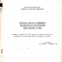 10970.pdf
Position: 1640 (12 views)